Graph Theory — Introduction
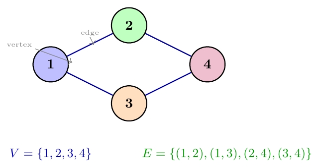
A graph is a mathematical structure used to model relationships between objects. The objects are called vertices (or nodes), and the relationships between them are called edges. A graph $G$ is written as $G = (V, E)$, where $V$ is the set of vertices and $E$ is the set of edges.
Think of a graph as a map of cities connected by roads. Each city is a vertex. Each road connecting two cities is an edge. Using this map, we can answer questions like, "Is there a path from city A to city B?" or "What is the shortest route?"
Social Network: People are vertices. A friendship is an edge between two people.
Road Network: Intersections are vertices. Roads are edges.
Internet: Computers are vertices. Network cables or wireless links are edges.
Course Prerequisites: Courses are vertices. An edge from course A to B means A must be done before B.
Basic Definitions
Vertex, Edge, and Graph $G = (V, E)$
A vertex (plural: vertices) is a single point or node in a graph. A vertex set $V$ is the collection of all vertices. We write $|V|$ to mean the total number of vertices.
An edge connects two vertices. An edge set $E$ is the collection of all edges. Each edge is written as a pair $(u, v)$, meaning there is a connection between vertex $u$ and vertex $v$.
For example, in the graph $G = (V, E)$ where $V = \{1, 2, 3, 4\}$ and $E = \{(1,2), (1,3), (2,4), (3,4)\}$, there are 4 vertices and 4 edges.
Directed vs. Undirected Graph
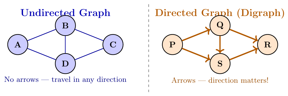
In an undirected graph, edges have no direction. If there is an edge between $u$ and $v$, you can go from $u$ to $v$ AND from $v$ to $u$. The edge $(u, v)$ and $(v, u)$ are the same edge. Think of a two-way road between two cities, you can drive in either direction.
In a directed graph (also called a digraph), every edge has a direction, shown by an arrow. Edge $(u, v)$ means you can go from $u$ to $v$, but NOT necessarily from $v$ to $u$. Think of a one-way road: you can only drive in one direction.
Weighted vs. Unweighted Graph
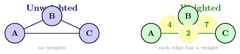
In an unweighted graph, all edges are equal. We only care if an edge exists or not. In a weighted graph, each edge has a number called a weight (or cost). This weight can represent distance, time, cost, or capacity. For example, in a road map, the weight on each edge might be the distance in kilometres between two cities.
Degree, In-Degree, and Out-Degree
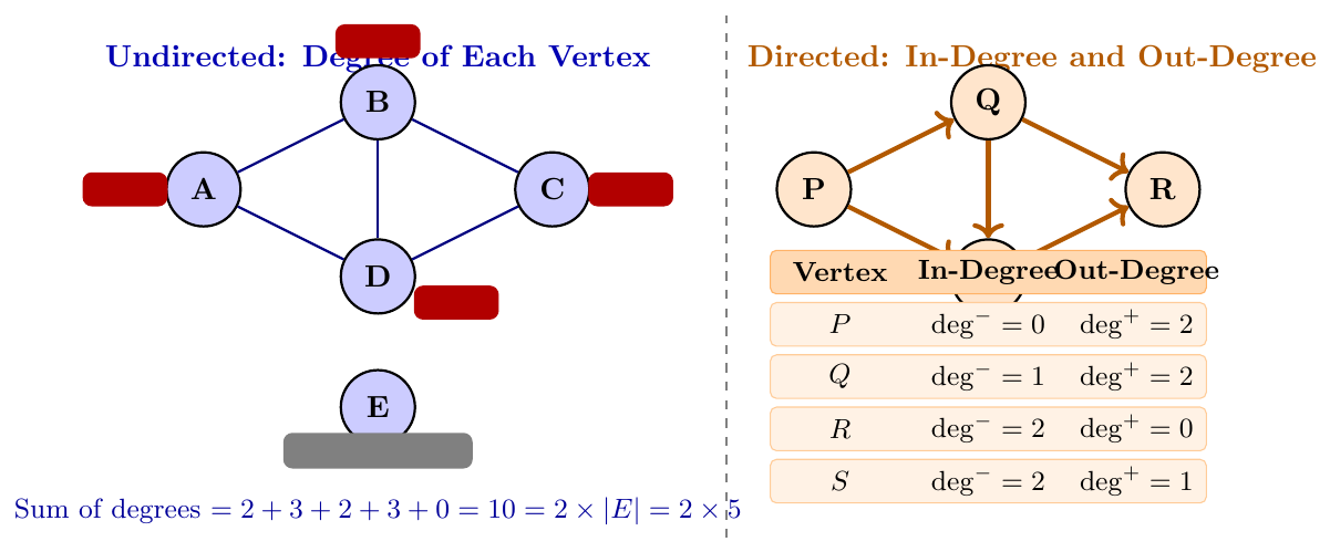
The degree of a vertex $v$ in an undirected graph is the number of edges connected to $v$. It is written as $\deg(v)$. A vertex with degree 0 is called an isolated vertex. A vertex with degree 1 is called a leaf or pendant vertex.
In a directed graph, each vertex $v$ has two degree values:
In-degree $(\deg^-(v))$: number of edges coming into $v$ (arrows pointing to $v$).
Out-degree $(\deg^+(v))$: number of edges going out of $v$ (arrows pointing away from $v$).
Handshaking Lemma
The Handshaking Lemma states that for any undirected graph $G = (V, E)$, \[ \sum_{v \in V} \deg(v) = 2|E| \] The sum of degrees of all vertices equals twice the number of edges. This is because every edge contributes exactly 2 to the total degree sum: one for each of its two endpoints. Counting degrees is like counting handshakes at a party: each handshake is counted once by each participant, so total counts = twice the handshakes.
Useful consequence: The number of vertices with odd degree is always even in any graph.
In the undirected graph above with vertices A(deg=2), B(deg=3), C(deg=2), D(deg=3), E(deg=0): \[ \sum \deg(v) = 2 + 3 + 2 + 3 + 0 = 10 = 2 \times 5 = 2|E| \] The graph has 5 edges. Twice 5 is 10. Confirmed.
Also, vertices with odd degree are B and D. That is 2 vertices, an even count. This is always true.
Complete Graph $K_n$
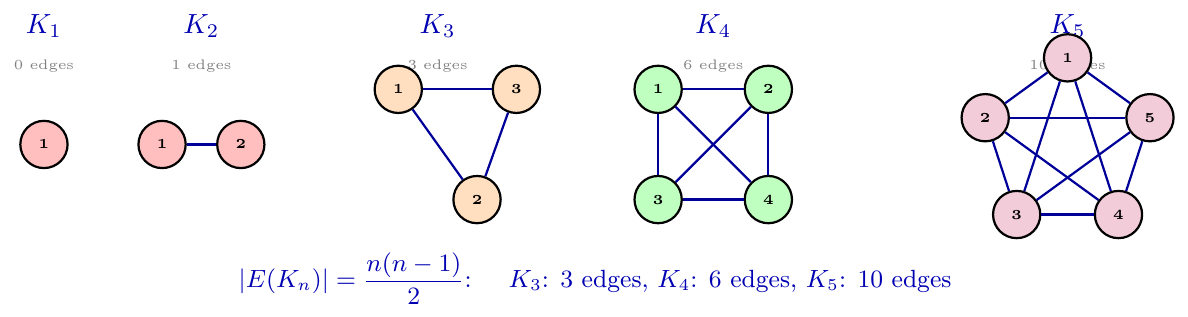
A complete graph $K_n$ is an undirected graph with $n$ vertices where every pair of distinct vertices is connected by exactly one edge. There is an edge between every possible pair.
The number of edges in $K_n$ is \[ |E| = \binom{n}{2} = \frac{n(n-1)}{2} \] because we choose 2 vertices from $n$ vertices for each edge. Also, every vertex in $K_n$ has degree $n-1$, since each vertex connects to all other $n-1$ vertices.
Directed Acyclic Graph (DAG)
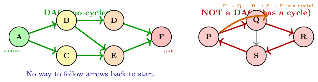
A DAG is a directed graph that has no directed cycles. That means, starting from any vertex, if you follow directed edges, you can never come back to the starting vertex. DAGs are used to represent dependencies, like course prerequisites, build systems, or scheduling tasks where some tasks must be done before others.
Key property: A DAG always has at least one vertex with in-degree 0 (no one points to it), called a source, and at least one vertex with out-degree 0 (it points to no one), called a sink.
Tree as a Special Graph
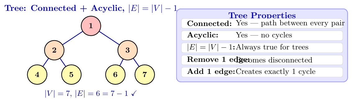
A tree is a special graph that satisfies all three of these properties simultaneously:
Undirected: edges have no direction.
Connected: there is a path between every pair of vertices.
Acyclic: there are no cycles.
From these three properties, a very important relationship follows automatically: \[ |E| = |V| - 1 \] A tree with $n$ vertices always has exactly $n-1$ edges. Remove any one edge and the tree becomes disconnected. Add any one edge and you create exactly one cycle.
Start with a single vertex (0 edges). Each time we add a new vertex to a tree, we must add exactly 1 edge to connect it (adding more than one edge would either create a cycle or disconnect something). So, after adding $n-1$ vertices to the first vertex, we have added $n-1$ edges total. Hence $|E| = |V| - 1 = n - 1$.
Connected Graph and Connected Components
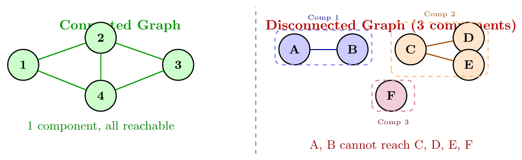
An undirected graph is called connected if there is a path between every pair of vertices. That means you can reach any vertex from any other vertex by following edges.
A graph that is NOT connected is called disconnected. In a disconnected graph, there are groups of vertices that are isolated from each other. Each such group is called a connected component.
Formally, a connected component is a maximal set of vertices such that every pair of vertices in the set is connected by some path, and no vertex outside the set is connected to any vertex inside it.
Think of a telephone network. If every phone can call every other phone (directly or through relays), the network is connected. If some phones are cut off from the rest, those isolated phones form a separate component.
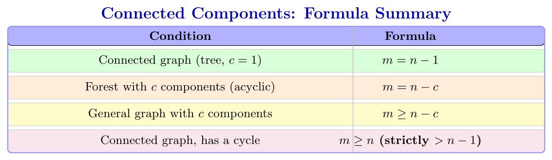
A connected undirected graph with $n$ vertices needs at least $n - 1$ edges. This minimum is achieved exactly when the graph is a tree. \[ \text{connected graph:} \quad |E| \ge n - 1 \] Why: To connect $n$ vertices into a single group, we need enough edges to link every vertex, directly or indirectly, to every other. The most economical way (using the fewest edges) is a tree structure with exactly $n-1$ edges. Fewer than $n-1$ edges can never connect $n$ vertices, because each edge can merge at most 2 previously separate components into 1, so we need at least $n-1$ merging steps.
For an undirected graph with $n$ vertices, $m$ edges, and $c$ connected components, IF the graph is acyclic (a forest): \[ m = n - c \] This generalizes the tree formula ($|E| = |V| - 1$, i.e., $c=1$) to the case of multiple components. Each component, being a tree, contributes (its own vertices $-1$) edges, and summing over all components gives $n - c$ total edges.
If the graph is not necessarily acyclic, then instead we only know: \[ m \ge n - c \] with equality holding if and only if every component is a tree (no cycles anywhere).
A forest has $n = 20$ vertices and $c = 5$ connected components (5 separate trees). The total number of edges is: \[ m = n - c = 20 - 5 = 15 \]
Now suppose instead we are told a general (not necessarily acyclic) graph has $n = 20$ vertices, $c = 5$ components, and $m = 18$ edges. Since $m = 18 > n - c = 15$, this graph has $18 - 15 = 3$ "extra" edges, meaning at least one component contains a cycle.
Strongly Connected and Weakly Connected (Directed Graphs)
A directed graph is called strongly connected if for every pair of vertices $u$ and $v$, there is a directed path from $u$ to $v$ and a directed path from $v$ to $u$. In simple words, you can reach every vertex from every other vertex by following the directed edges.
A Strongly Connected Component (SCC) is a maximal subset of vertices that are all mutually reachable from each other.
A directed graph is called weakly connected if the underlying undirected graph (obtained by ignoring all arrow directions) is connected. So weakly connected means connected if we pretend all edges are two-way. Weakly connected does NOT require paths in both directions.
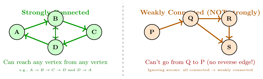
For any directed graph: \[ \text{Strongly Connected} \implies \text{Weakly Connected} \] But the reverse is NOT true, weakly connected does not imply strongly connected (as shown in the example above).
Special case: If a directed graph has no edges at all between any pair of vertices (i.e., it's just isolated vertices), it is neither strongly nor weakly connected (unless it has just 1 vertex, in which case it is trivially both).
Consider a directed graph with vertices $\{P, Q, R, S\}$ and edges: $P \to Q$, $Q \to R$, $R \to S$, $Q \to S$.
Check strong connectivity: Can we go from $S$ back to $P$? There is no outgoing edge from $S$ at all (out-degree of $S$ is 0). So $S$ cannot reach any other vertex. NOT strongly connected.
Check weak connectivity: Ignoring directions, the underlying undirected graph has edges $P-Q$, $Q-R$, $R-S$, $Q-S$. This connects all 4 vertices into one component. Weakly connected: YES.
Walk, Trail, Circuit, Path, and Cycle
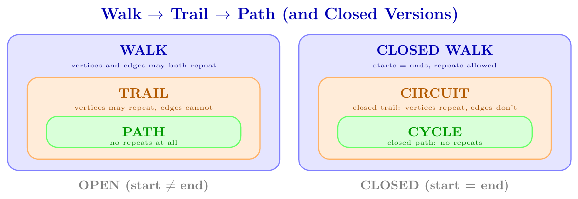
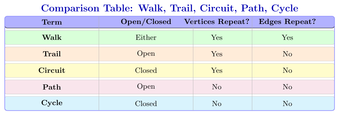
A walk is a finite alternating sequence of vertices and edges, where consecutive vertices are joined by the edge between them. Both vertices and edges are allowed to repeat freely in a walk. The length of a walk is the number of edges covered in it.
A walk is called open if its length is greater than 0 and the starting and ending vertices are different. A walk is called closed if its length is greater than 0 and the starting and ending vertices are the same. A walk of length 0 (a single vertex, no edges) is called a trivial walk.
Think of a person wandering through a city with no particular destination in mind. They may cross the same street multiple times, or pass through the same square again and again. This unrestricted wandering, where nothing is off-limits to repeat, is exactly a walk.
A trail is an open walk in which vertices may repeat, but edges are not allowed to repeat. Think of a trail as a walk with one extra restriction: once you have used a particular road, you cannot use that exact road again, but you are still allowed to revisit the same junction.
A circuit is a closed walk in which vertices may repeat, but edges are not allowed to repeat. In other words, a circuit is simply a trail that returns to its starting vertex. A closed trail is called a circuit.
A path is an open walk in which neither vertices (except possibly the starting and ending vertex) nor edges are allowed to repeat. This is the strictest form of an open walk: every vertex is visited at most once, so naturally every edge is also used at most once (since repeating an edge would force repeating a vertex).
A cycle is a closed walk in which neither vertices nor edges are allowed to repeat, except that the starting and ending vertex is the same. In other words, a cycle is a closed path. A closed path is called a cycle.
Since a path never repeats vertices, it automatically never repeats edges either. So:
Every path is a trail, but every trail need not be a path (a trail is allowed to repeat vertices, a path is not).
Every cycle is a circuit, but every circuit need not be a cycle (a circuit is allowed to repeat vertices, a cycle is not).
For directed graphs, we simply place the word “directed” in front of each of these terms: directed walk, directed trail, directed circuit, directed path, directed cycle. The same repetition rules apply, just following the direction of the arrows.
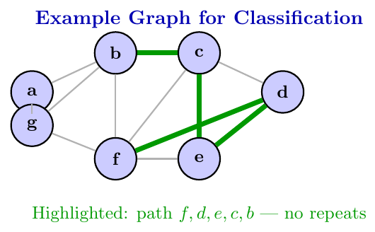
Consider a graph with vertices $\{a, b, c, d, e, f, g\}$. Classify each of the following vertex sequences.
$a, b, g, f, c, b$: Open (starts at $a$, ends at $b$). Vertex $b$ repeats, but no edge repeats. This is a trail (not a path, since vertex $b$ is repeated).
$b, g, f, c, b, g, a$: Open. Both vertices ($b$, $g$) and possibly edges repeat here (edge $b$–$g$ used twice). This is just a general walk (not even a trail, since an edge repeats).
$c, e, f, c$: Closed (starts and ends at $c$). No vertex or edge repeats other than the start/end vertex $c$. This is a cycle.
$c, e, f, c, e$: Open (starts at $c$, ends at $e$). If no edge repeats but vertices $c$ and $e$ appear more than once internally, this is a trail.
$a, b, f, a$: If there is no edge directly between $f$ and $a$ in the graph, this sequence is not a valid walk at all, since consecutive vertices must be joined by an edge.
$f, d, e, c, b$: Open, no vertex repeats, no edge repeats. This is a path.
Consider a directed graph with vertices $\{u, v, w, x, y\}$ and directed edges $x\to v$, $v \to y$, $y \to w$, $w \to v$, $x \to u$, $u \to x$.
Sequence $x, v, y, w, v$: Check each consecutive pair has a directed edge: $x\to v$ ✓, $v \to y$ ✓, $y \to w$ ✓, $w \to v$ ✓. This is a valid directed walk of length 4. Vertex $v$ repeats, so it is not a directed path; since start ($x$) $\ne$ end ($v$), it is not a directed cycle either. If no edge repeats, it is a directed trail.
Sequence $x, u, v, y, x$: Check $u \to v$: no such directed edge exists (only $u \to x$ exists from $u$). This is not a valid directed walk at all.
Havel–Hakimi Theorem
Given a list of numbers, a natural question is: can we build a simple undirected graph where these numbers are exactly the degrees of the vertices? Such a sequence is called a graphical sequence (or graphic sequence). Not every sequence of numbers is graphical; some sequences simply cannot correspond to any real graph, however hard we try to draw edges. The Havel–Hakimi algorithm gives us a step-by-step method to test this, without needing to try every possible graph.
A degree sequence $d_1 \ge d_2 \ge \cdots \ge d_n \ge 0$ (sorted in non-increasing order) is graphical if and only if the sequence \[ (d_2 - 1, d_3 - 1, \ldots, d_{d_1+1} - 1, d_{d_1+2}, \ldots, d_n) \] obtained by removing the largest value $d_1$ and subtracting 1 from the next $d_1$ largest entries, is also graphical.
In plain words: take the vertex with the highest degree, say $d_1$. Connect it to the $d_1$ next-highest-degree vertices (this is always possible, and always the safest choice). Once that vertex is fully connected, remove it from the list, and reduce the degree of each vertex it was connected to by 1 (since each of those vertices has now used up one of its edges). Repeat this process on the smaller sequence.
Think of $n$ people, each wanting a specific number of handshakes ($d_1, d_2, \ldots, d_n$). The greedy idea is: take the person who wants the most handshakes, and simply pair them up with the next most eager people, since that is always a safe, non-wasteful choice. Once that person's handshakes are all arranged, we remove them from the room and reduce the remaining handshake counts of the people they shook hands with by 1 each (since those handshakes have already happened). We keep repeating this with the reduced list.
If at any point during this process we get a negative number in the list, it means the sequence is not graphical, impossible to satisfy. If we can reduce the whole list down to all zeros, the sequence is graphical.
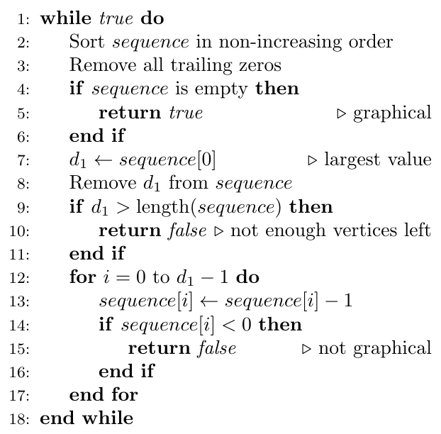
At each step of the algorithm, sort the sequence in non-increasing order first. Then check:
If all remaining values are 0, the sequence is graphical. Stop.
If the largest value $d_1$ is greater than the number of remaining entries (excluding itself), the sequence is NOT graphical. Stop (there simply aren't enough other vertices to connect to).
If subtracting 1 produces any negative value, the sequence is NOT graphical. Stop.
Otherwise, repeat the reduction step on the new sequence.
Algorithm: Havel-Hakimi(sequence)
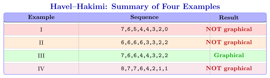
Step 1: Sequence: $7, 6, 5, 4, 4, 3, 2, 0$. Largest value is 7. Remove it, and subtract 1 from the next 7 entries. \[ 6-1, 5-1, 4-1, 4-1, 3-1, 2-1, 0-1 \] The last entry becomes $0 - 1 = -1$, which is negative.
Conclusion: Since a negative value appears, the sequence $7, 6, 5, 4, 4, 3, 2, 0$ is NOT graphical.
Intuition: A vertex wanting degree 0 cannot be connected to at all, but the vertex with degree 7 needs to connect to all 7 remaining vertices, forcing a connection with the degree-0 vertex. This is a direct contradiction.
Step 1: Sequence: $6, 6, 6, 6, 3, 3, 2, 2$. Largest value is 6. Remove it, subtract 1 from the next 6 entries. \[ 6-1, 6-1, 6-1, 3-1, 3-1, 2-1, \; 2 \] New sequence (before sorting): $5, 5, 5, 2, 2, 1, 2$. Sorted: $5, 5, 5, 2, 2, 2, 1$.
Step 2: Largest value is 5. Remove it, subtract 1 from the next 5 entries. \[ 5-1, 5-1, 2-1, 2-1, 2-1, \; 1 \] New sequence (before sorting): $4, 4, 1, 1, 1, 1$. Sorted: $4, 4, 1, 1, 1, 1$.
Step 3: Largest value is 4. Remove it, subtract 1 from the next 4 entries. \[ 4-1, 1-1, 1-1, 1-1, \; 1 \] New sequence (before sorting): $3, 0, 0, 0, 1$. Sorted: $3, 1, 0, 0, 0$.
Step 4: Largest value is 3. Remove it, subtract 1 from the next 3 entries. \[ 1-1, 0-1, 0-1 \] The entry $0 - 1 = -1$ is negative.
Conclusion: The sequence $6, 6, 6, 6, 3, 3, 2, 2$ is NOT graphical.
Step 1: Sequence: $7, 6, 6, 4, 4, 3, 2, 2$. Largest value is 7, and there are exactly 7 remaining entries, so this is valid (not too large). Subtract 1 from all 7 remaining entries. \[ 6-1, 6-1, 4-1, 4-1, 3-1, 2-1, 2-1 \] New sequence: $5, 5, 3, 3, 2, 1, 1$. Already sorted.
Step 2: Largest value is 5. Remove it, subtract 1 from the next 5 entries. \[ 5-1, 3-1, 3-1, 2-1, 1-1, \; 1 \] New sequence (before sorting): $4, 2, 2, 1, 0, 1$. Sorted: $4, 2, 2, 1, 1, 0$.
Step 3: Largest value is 4. Remove it, subtract 1 from the next 4 entries. \[ 2-1, 2-1, 1-1, 1-1, \; 0 \] New sequence (before sorting): $1, 1, 0, 0, 0$. Sorted: $1, 1, 0, 0, 0$.
Step 4: Drop trailing zeros: $1, 1$. Largest value is 1. Remove it, subtract 1 from the next 1 entry. \[ 1 - 1 = 0 \] New sequence: $0$.
Step 5: Drop trailing zero. Sequence is now empty.
Conclusion: We reached an empty sequence (all zeros) without ever hitting a negative number. So $7, 6, 6, 4, 4, 3, 2, 2$ IS graphical.
Step 1: Sequence: $8, 7, 7, 6, 4, 2, 1, 1$. The largest value is 8, but there are only 7 remaining entries in the sequence.
\[ d_1 = 8 > \text{(number of remaining entries)} = 7 \]
Conclusion: Since the largest degree (8) exceeds the number of other vertices available to connect to (only 7 remain), it is impossible for this vertex to achieve degree 8 in a simple graph (no self-loops or multi-edges allowed). So $8, 7, 7, 6, 4, 2, 1, 1$ is NOT graphical.
Intuition: With only 8 vertices total, the maximum possible degree for any single vertex is $8 - 1 = 7$ (connecting to every other vertex). A degree of 8 is simply impossible here.
Graph Representations
The same graph can be stored in a computer in different ways. The choice of representation affects:
How much memory we use.
How fast we can check if an edge exists.
How fast we can traverse all neighbours of a vertex.
How fast graph algorithms run in total.
The two most common representations are the adjacency matrix and the adjacency list.
Adjacency Matrix
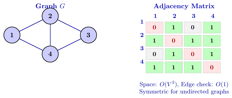
An adjacency matrix is a 2D array (matrix) of size $|V| \times |V|$. For a graph with $|V| = n$ vertices numbered $1$ to $n$: \[ A[i][j] = \begin{cases} 1 & \text{if there is an edge from vertex } i \text{ to vertex } j \\ 0 & \text{otherwise} \end{cases} \] For a weighted graph, we store the weight instead of 1. For an undirected graph, the matrix is always symmetric, meaning $A[i][j] = A[j][i]$.
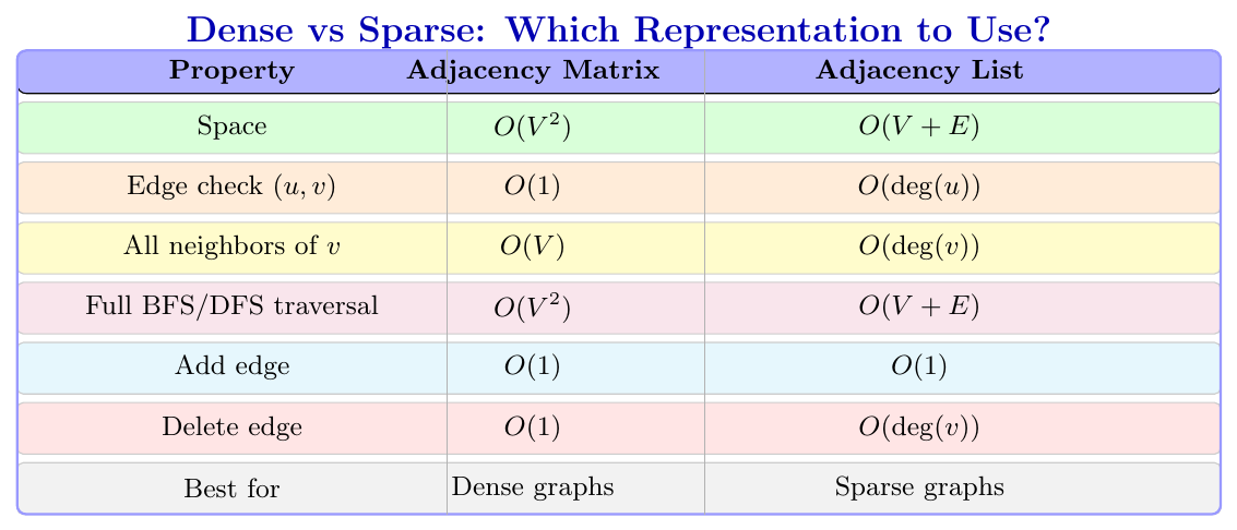
Space: $O(V^2)$, regardless of the number of edges.
Edge check: $O(1)$, since $A[u][v]$ gives the answer directly.
Finding all neighbours of $v$: $O(V)$, since we must scan the entire row $v$.
Adjacency List
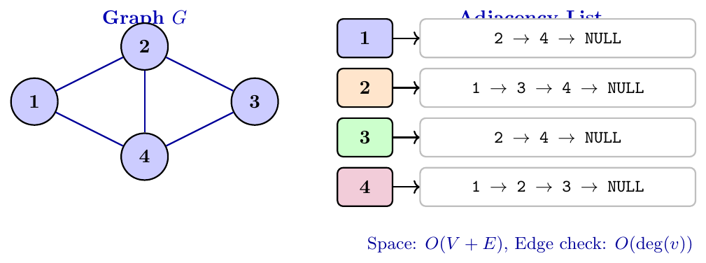
An adjacency list stores, for each vertex $v$, a list of all vertices adjacent to $v$ (its neighbours). We can implement this as an array of linked lists, or as an array of Python lists.
Space: $O(V + E)$, since we store $|V|$ list headers and $2|E|$ total entries (each edge appears in two lists for undirected graph, or $|E|$ entries total for directed).
Edge check: $O(\deg(v))$, we must scan the list of $v$ to see if $u$ is in it.
Finding all neighbours of $v$: $O(\deg(v))$, simply iterate the list.
Total traversal: $O(V + E)$, visiting all vertices and all their edges.
Dense vs. Sparse Graphs
A dense graph has many edges, close to the maximum possible. A complete graph $K_n$ is the densest possible, with $n(n-1)/2$ edges. For dense graphs, $|E| \approx |V|^2$, so adjacency matrix wastes little space and makes edge checks very fast.
A sparse graph has few edges, much less than the maximum. For sparse graphs, $|E| \ll |V|^2$, often $|E| \approx |V|$ or $|E| \approx |V| \log |V|$. Adjacency list is much better here because the matrix would be mostly empty zeros, wasting memory.
Facebook network: billions of users (vertices) but each person has only a few thousand friends (edges). This is very sparse. $|E| \ll |V|^2$. Use adjacency list.
A 5-city road network where every city is connected to every other: $K_5$, 10 edges. Dense for 5 nodes. Matrix is fine here.
Flight network: thousands of airports, but not all airports connect to each other. Sparse. Use adjacency list.
A graph algorithm on a 1000-vertex dense graph: matrix allows $O(1)$ edge check, which is critical here.
When we run graph traversal algorithms like BFS or DFS:
Using adjacency matrix: For each vertex $v$, we scan its entire row to find neighbours. This takes $O(V)$ per vertex, and with $V$ vertices total, the whole traversal takes $O(V^2)$.
Using adjacency list: For each vertex $v$, we only look at the neighbours in its list. The total work across all vertices is proportional to the total number of entries in all lists, which equals $2|E|$ (each edge appears twice for undirected). So total traversal takes $O(V + E)$.
For sparse graphs where $|E| \ll |V|^2$, the adjacency list traversal $O(V+E)$ is much faster than matrix traversal $O(V^2)$.
Consider a sparse graph with $|V| = 1000$ and $|E| = 2000$ (each vertex connects to 2 others on average).
Adjacency matrix BFS/DFS: $O(V^2) = O(1000^2) = O(1{,}000{,}000)$ operations.
Adjacency list BFS/DFS: $O(V+E) = O(1000 + 2000) = O(3000)$ operations.
Adjacency list is about 333 times faster here. This difference becomes even larger for bigger sparse graphs.