Searching and Sorting
Searching means finding whether a given value (the key) is present in a collection, and if so, where. Sorting means rearranging the elements of a collection into increasing (or decreasing) order. The two are closely linked. Sorting costs time once, but afterwards searching becomes much faster (binary search instead of linear search).
Think of a library. If the books are thrown in a heap, you must check every book to find one title (linear search). If the books are arranged alphabetically, you open the middle shelf and decide to go left or right (binary search). Arranging the books is sorting.
In this chapter all sorting algorithms are comparison-based: they learn about the order of elements only by comparing two elements at a time.
Stable: Equal elements keep their original relative order. If two records have the same key and record $X$ comes before record $Y$ in the input, then $X$ still comes before $Y$ in the output. This matters when sorting by multiple keys (sort by marks, then by name).
In-place: The algorithm uses only $O(1)$ extra memory (some books also allow $O(\log n)$ for recursion stack). It sorts inside the same array.
Adaptive: The algorithm runs faster when the input is already partly sorted. For example, it takes $O(n)$ time on a sorted array.
Online: The algorithm can sort the list as new elements keep arriving, without seeing the whole input first.
In an array $A[0..n-1]$, a pair of positions $(i, j)$ with $i < j$ and $A[i] > A[j]$ is called an inversion. It is a pair that is in the wrong order.
A sorted array has $0$ inversions.
A reverse-sorted array of distinct elements has the maximum, $\dbinom{n}{2} = \dfrac{n(n-1)}{2}$ inversions.
Every swap of two adjacent elements changes the inversion count by exactly $1$.
Therefore any algorithm that moves elements only by adjacent swaps (bubble sort, insertion sort) needs at least as many swaps or shifts as the number of inversions.
Array $A = [3, 1, 4, 2]$.
$(3,1)$: inversion, since $3 > 1$.
$(3,2)$: inversion.
$(4,2)$: inversion.
$(3,4)$, $(1,4)$, $(1,2)$: not inversions.
Total inversions $= 3$. The maximum possible for $n=4$ is $\frac{4 \cdot 3}{2} = 6$.
Search Algorithms
Linear Search
Linear search checks the elements one by one from the beginning, until the key is found or the array ends. It does not need the array to be sorted. It works on arrays and linked lists.
Best case: key at the first position, $1$ comparison, $\Theta(1)$.
Worst case: key at the last position or absent, $n$ comparisons, $\Theta(n)$.
Average case: if the key is present and equally likely at any position, $\dfrac{1+2+\cdots+n}{n} = \dfrac{n+1}{2}$ comparisons, $\Theta(n)$.
Algorithm: Linear-Search(A, n, key)
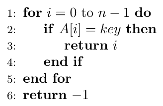
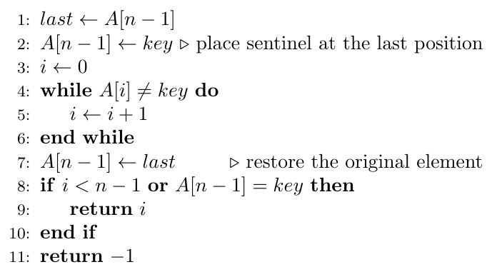
In the normal loop, every iteration does two tests: “is $i < n$?” and “is $A[i] = key$?”. In sentinel search, we place the key itself at the end, $A[n] = key$, so that the loop is guaranteed to stop. Now only one test per iteration is needed. After the loop, we check whether the position found is $< n$. The complexity is still $\Theta(n)$, but the constant becomes smaller. The algorithm needs one extra slot in the array.
Algorithm: Sentinel-Linear-Search(A, n, key)
def linear_search(a, key):
    for i in range(len(a)):
        if a[i] == key:
            return i
    return -1


def sentinel_search(a, key):
    n = len(a)
    last = a[n - 1]
    a[n - 1] = key              # sentinel
    i = 0
    while a[i] != key:          # only ONE test per iteration
        i += 1
    a[n - 1] = last             # restore
    if i < n - 1 or last == key:
        return i
    return -1


print(linear_search([7, 3, 9, 4], 9))     # 2
print(sentinel_search([7, 3, 9, 4], 5))   # -1
Binary Search
Binary search needs a sorted array (with random access). It compares the key with the middle element.
If the key equals the middle element, we are done.
If the key is smaller, the key can only be in the left half, so we discard the right half.
If the key is larger, the key can only be in the right half, so we discard the left half.
Each step throws away half of the remaining elements. After $k$ steps, at most $n/2^k$ elements remain. The search ends when this becomes less than $1$, i.e., after about $\log_2 n$ steps.
Your friend thinks of a number between $1$ and $1000$. You ask “Is it more than 500?” and he answers yes or no. Every answer halves the possibilities. In at most $10$ questions ($2^{10} = 1024 \ge 1000$) you find the number. Binary search is exactly this game.
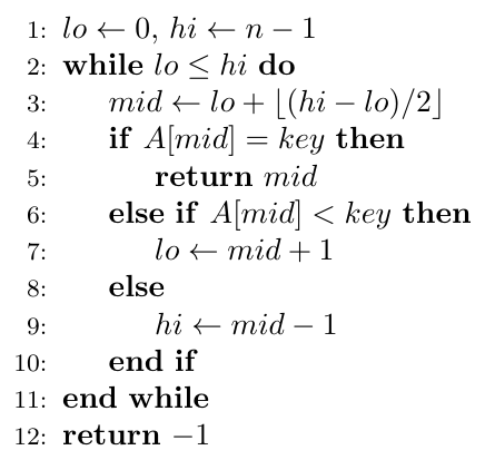
Algorithm: Binary-Search-Iterative(A, n, key)
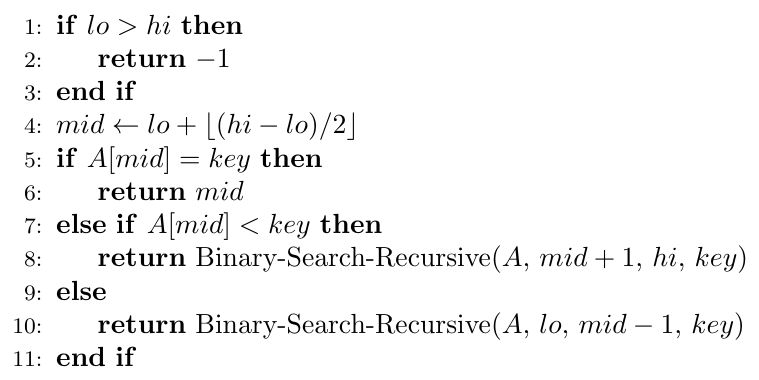
Algorithm: Binary-Search-Recursive(A, lo, hi, key)
BinarySearch(A, n, key):
lo = 0, hi = n - 1
while lo <= hi:
mid = lo + (hi - lo) / 2
if A[mid] == key: return mid
else if A[mid] < key: lo = mid + 1
else: hi = mid - 1
return -1
One comparison, then one subproblem of half the size: \[ T(n) = T(n/2) + \Theta(1), \qquad T(1) = \Theta(1) \] By Master theorem ($a=1$, $b=2$, $n^{\log_2 1} = 1 = \Theta(f(n))$, Case 2): $T(n) = \Theta(\log n)$.
Best case: the key is at the first middle, $\Theta(1)$.
Worst and average case: $\Theta(\log n)$.
Space: iterative $O(1)$; recursive $O(\log n)$ for the call stack.
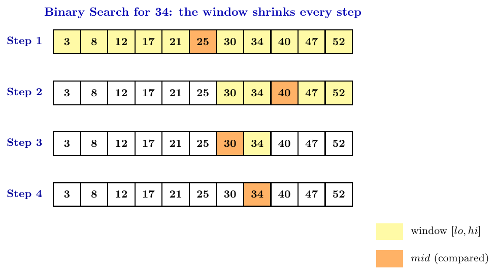
$A = [3, 8, 12, 17, 21, 25, 30, 34, 40, 47, 52]$ (indices $0$ to $10$, $n=11$).
Iteration 1: $lo=0$, $hi=10$, $mid=5$, $A[5]=25 < 34$, so $lo = 6$.
Iteration 2: $lo=6$, $hi=10$, $mid=8$, $A[8]=40 > 34$, so $hi = 7$.
Iteration 3: $lo=6$, $hi=7$, $mid=6$, $A[6]=30 < 34$, so $lo = 7$.
Iteration 4: $lo=7$, $hi=7$, $mid=7$, $A[7]=34$. Found at index $7$.
Total iterations $= 4 = \lfloor \log_2 11 \rfloor + 1$.
Counting convention: one comparison per iteration (the three-way test $A[mid]$ against the key). GATE questions usually count iterations this way, but always read the question.
Worst case (successful or unsuccessful): $\lfloor \log_2 n \rfloor + 1$.
For $n = 2^k - 1$ (a perfect decision tree): the key at the first middle needs $1$ comparison, the two keys at the next level need $2$ each, the four keys at the next level need $3$ each, and so on. In general, $2^{j-1}$ keys need exactly $j$ comparisons.
Average successful search for $n = 2^k - 1$: \[ \frac{\sum_{j=1}^{k} j \cdot 2^{j-1}}{n} = \frac{(k-1)2^k + 1}{2^k - 1} \] which is about $\log_2 n - 1$ for large $n$.
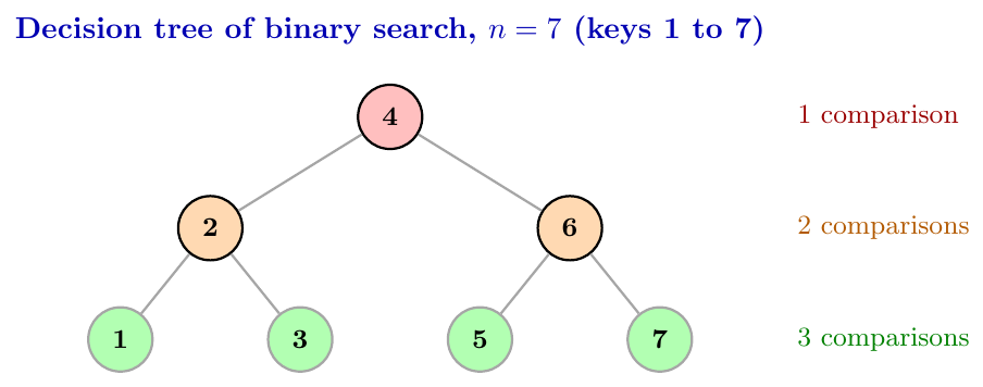
Level 1 has $1$ key (1 comparison), level 2 has $2$ keys (2 comparisons each), level 3 has $4$ keys (3 each), level 4 has $8$ keys (4 each). \[ \text{Total} = 1(1) + 2(2) + 4(3) + 8(4) = 1 + 4 + 12 + 32 = 49 \] Average for a successful search $= \dfrac{49}{15} \approx 3.27$. Worst case $= \lfloor \log_2 15 \rfloor + 1 = 4$.
Needs a sorted array. On an unsorted array the answer is meaningless.
Needs random access ($O(1)$ access to the middle). On a linked list, reaching the middle costs $O(n)$, so binary search loses its advantage.
Overflow: In fixed-width integers, $mid = (lo + hi)/2$ can overflow. Use $mid = lo + (hi - lo)/2$. (Python integers do not overflow, but the habit is important.)
Duplicates: Plain binary search returns some index of the key, not necessarily the first or last. To find the first occurrence (lower bound), do not stop at equality; keep searching on the left.
Off-by-one: The loop condition $lo \le hi$ with updates $mid \pm 1$ must go together. Mixing $lo < hi$ with $hi = mid$ is a different, valid style, but mixing the two styles by mistake gives infinite loops.
Modified version, interpolation search: instead of the middle, probe at $lo + \dfrac{(key - A[lo])(hi - lo)}{A[hi] - A[lo]}$. For uniformly distributed keys the average is $O(\log\log n)$, but the worst case is $O(n)$.
def binary_search(a, key):
    lo, hi = 0, len(a) - 1
    while lo <= hi:
        mid = lo + (hi - lo) // 2
        if a[mid] == key:
            return mid
        elif a[mid] < key:
            lo = mid + 1
        else:
            hi = mid - 1
    return -1


def binary_search_rec(a, lo, hi, key):
    if lo > hi:
        return -1
    mid = lo + (hi - lo) // 2
    if a[mid] == key:
        return mid
    if a[mid] < key:
        return binary_search_rec(a, mid + 1, hi, key)
    return binary_search_rec(a, lo, mid - 1, key)


def lower_bound(a, key):
    """Index of the FIRST element >= key (works with duplicates)."""
    lo, hi = 0, len(a)
    while lo < hi:
        mid = lo + (hi - lo) // 2
        if a[mid] < key:
            lo = mid + 1
        else:
            hi = mid            # do not stop: keep looking left
    return lo


def count_iterations(a, key):
    lo, hi, steps = 0, len(a) - 1, 0
    while lo <= hi:
        steps += 1
        mid = lo + (hi - lo) // 2
        if a[mid] == key:
            return steps
        elif a[mid] < key:
            lo = mid + 1
        else:
            hi = mid - 1
    return steps


A = [3, 8, 12, 17, 21, 25, 30, 34, 40, 47, 52]
print(binary_search(A, 34))        # 7
print(count_iterations(A, 34))     # 4
print(lower_bound([1, 2, 2, 2, 3], 2))   # 1
Binary Search on the Answer
Sometimes there is no sorted array, but the answer itself lies in a range of numbers and has a monotone yes/no property. For example, if speed $k$ works, then every speed larger than $k$ also works. Such a predicate looks like \[ \underbrace{\text{No, No, No,}}_{\text{infeasible}} \; \underbrace{\text{Yes, Yes, Yes}}_{\text{feasible}} \] We binary search for the first Yes. Each step calls a feasibility check $\text{feasible}(mid)$ costing $C$, so the total cost is $O(C \cdot \log(\text{range size}))$.
Template: $lo$ = smallest possible answer, $hi$ = a value that is surely feasible. While $lo < hi$: $mid = lo + (hi-lo)/2$; if $\text{feasible}(mid)$ then $hi = mid$ else $lo = mid + 1$. At the end $lo$ is the answer.
Find $\lfloor \sqrt{x} \rfloor$ for $x = 50$. The largest $m$ with $m^2 \le x$. Search $m \in [0, 50]$ with predicate “$m^2 > x$” (the first Yes is $\lfloor\sqrt{x}\rfloor + 1$). Since $7^2 = 49 \le 50 < 64 = 8^2$, the answer is $7$. This takes about $\log_2 50 \approx 6$ steps instead of $7$ linear steps, and for $x = 10^{18}$ it takes about $60$ steps instead of $10^9$.
Piles $= [3, 6, 7, 11]$ bananas, and we have $h = 8$ hours. Each hour we eat from one pile at speed $k$ (a pile of $p$ takes $\lceil p/k \rceil$ hours). Find the minimum integer $k$ that finishes in $h$ hours.
Feasible$(k)$ means $\sum \lceil p_i/k \rceil \le 8$.
$k=4$: $1 + 2 + 2 + 3 = 8 \le 8$, feasible.
$k=3$: $1 + 2 + 3 + 4 = 10 > 8$, not feasible.
Since feasibility is monotone in $k$, binary search over $k \in [1, 11]$ gives the minimum $k = 4$.
import math

def isqrt_floor(x):
    lo, hi = 0, x + 1               # first m with m*m > x
    while lo < hi:
        mid = lo + (hi - lo) // 2
        if mid * mid > x:           # feasible (Yes)
            hi = mid
        else:
            lo = mid + 1
    return lo - 1


def min_speed(piles, h):
    def feasible(k):
        return sum(math.ceil(p / k) for p in piles) <= h

    lo, hi = 1, max(piles)
    while lo < hi:
        mid = lo + (hi - lo) // 2
        if feasible(mid):
            hi = mid
        else:
            lo = mid + 1
    return lo


print(isqrt_floor(50))                 # 7
print(min_speed([3, 6, 7, 11], 8))     # 4
Basic (Quadratic) Sorting
Selection Sort
Selection sort repeatedly selects the minimum element of the unsorted part and puts it at the front of the unsorted part. After pass $i$, the first $i$ positions hold the $i$ smallest elements in their final places.
Analogy: Arranging cards in hand by repeatedly picking the smallest card from the remaining pile and placing it next in a row.
Algorithm: Selection-Sort(A, n)
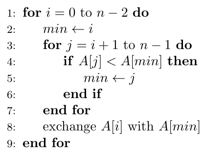
Pass 1: minimum of all $= 11$ (index 4). Swap with index 0: $[11, 25, 12, 22, 64]$. Comparisons: $4$.
Pass 2: minimum of $[25,12,22,64] = 12$. Swap with index 1: $[11, 12, 25, 22, 64]$. Comparisons: $3$.
Pass 3: minimum of $[25,22,64] = 22$. Swap with index 2: $[11, 12, 22, 25, 64]$. Comparisons: $2$.
Pass 4: minimum of $[25,64] = 25$, already at index 3. Self-swap (no change). Comparisons: $1$.
Total comparisons $= 4+3+2+1 = 10 = \frac{5 \cdot 4}{2}$. Swaps performed $= 4$ (only $3$ if we skip self-swaps).
Comparisons: always exactly $\dfrac{n(n-1)}{2}$, for every input (sorted, reversed or random). So best = average = worst $= \Theta(n^2)$.
Swaps: at most $n-1$, so $O(n)$. This is the minimum number of writes among the simple sorts, useful when writing to memory is expensive.
Not adaptive: a sorted array still costs $\Theta(n^2)$ comparisons.
In-place: yes, $O(1)$ extra space.
Not stable (in the swap form): the long-distance swap can jump an element over equal elements. Example: $[4_a, 4_b, 3]$. Pass 1 swaps $4_a$ with $3$ and gives $[3, 4_b, 4_a]$, so $4_a$ and $4_b$ are reversed.
Not online: it must see all elements to find the minimum.
Stable selection sort: instead of swapping, shift the elements between $i$ and $min$ one place to the right and insert the minimum at position $i$. This keeps equal elements in order, but now the writes become $O(n^2)$.
Bidirectional (double) selection sort: in each pass find both the minimum and the maximum and place them at the two ends. Passes halve, but comparisons stay $\Theta(n^2)$.
Heap sort is selection sort with a smarter way (a heap) of finding the minimum or maximum, reducing $\Theta(n^2)$ to $\Theta(n\log n)$.
def selection_sort(a):
    n = len(a)
    comparisons = swaps = 0
    for i in range(n - 1):
        m = i
        for j in range(i + 1, n):
            comparisons += 1
            if a[j] < a[m]:
                m = j
        if m != i:
            a[i], a[m] = a[m], a[i]
            swaps += 1
    return comparisons, swaps


def stable_selection_sort(a):
    n = len(a)
    for i in range(n - 1):
        m = i
        for j in range(i + 1, n):
            if a[j] < a[m]:          # strict: first minimum is chosen
                m = j
        key = a[m]
        while m > i:                 # shift instead of swap
            a[m] = a[m - 1]
            m -= 1
        a[i] = key


A = [64, 25, 12, 22, 11]
print(selection_sort(A), A)          # (10, 3) [11, 12, 22, 25, 64]
Bubble Sort
Bubble sort repeatedly walks through the array and compares adjacent elements. If a pair is in the wrong order, it swaps them. In each pass, the largest remaining element “bubbles up” to the end like an air bubble rising in water. After pass $i$, the last $i$ positions hold the $i$ largest elements in final places.
Algorithm: Bubble-Sort(A, n) — with early exit
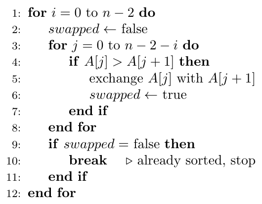
Pass 1 (4 comparisons): $(5,1)$ swap $\to [1,5,4,2,8]$; $(5,4)$ swap $\to [1,4,5,2,8]$; $(5,2)$ swap $\to [1,4,2,5,8]$; $(5,8)$ no swap. Result $[1,4,2,5,8]$, 3 swaps.
Pass 2 (3 comparisons): $(1,4)$ no; $(4,2)$ swap $\to [1,2,4,5,8]$; $(4,5)$ no. 1 swap.
Pass 3 (2 comparisons): $(1,2)$ no; $(2,4)$ no. No swap, so stop.
Total comparisons $= 4+3+2 = 9$. Total swaps $= 4 = $ number of inversions of the input ($(5,1),(5,4),(5,2),(4,2)$). Passes executed $= 3$ (two to sort, one to confirm).
Swaps $=$ number of inversions $I$ exactly (each swap fixes exactly one inversion).
Comparisons:
Without early exit: always $\dfrac{n(n-1)}{2}$.
With early exit: best case (sorted) $n-1$, worst case (reversed) $\dfrac{n(n-1)}{2}$.
Time: best $\Theta(n)$ (only with the early-exit flag), average and worst $\Theta(n^2)$.
Number of passes to sort $=$ maximum, over all elements, of the number of larger elements before it (how far an element must move left). Add one more pass if the early-exit flag version must confirm. In the example above: $2$ for the element $2$ (the larger elements $5$ and $4$ are before it), so $2$ passes sort it, plus $1$ confirming pass.
Stable: yes, because we swap only when $A[j] > A[j+1]$ strictly.
In-place: yes. Adaptive: yes, with the flag. Online: no.
Hare and tortoise behaviour: large elements near the front (“rabbits”) move to the end quickly, but small elements near the end (“turtles”) move left only one place per pass. A single small element at the end of an otherwise sorted array forces $n-1$ passes.
Early-exit flag (shown above) makes it adaptive: $\Theta(n)$ on sorted input.
Last-swap-position optimisation: remember the index of the last swap in a pass. Everything after it is already sorted, so the next pass only needs to go up to that index. Good for arrays whose tail is already sorted.
Cocktail shaker sort (bidirectional bubble sort): alternate passes left-to-right (pushes the largest to the end) and right-to-left (pushes the smallest to the front). It handles the “turtle” problem. Still $\Theta(n^2)$ worst case, stable, in-place.
def bubble_sort(a):
    n = len(a)
    comparisons = swaps = passes = 0
    for i in range(n - 1):
        swapped = False
        passes += 1
        for j in range(n - 1 - i):
            comparisons += 1
            if a[j] > a[j + 1]:
                a[j], a[j + 1] = a[j + 1], a[j]
                swaps += 1
                swapped = True
        if not swapped:
            break
    return comparisons, swaps, passes


def bubble_sort_last_swap(a):
    """Shrinks the range using the position of the last swap."""
    n = len(a)
    end = n - 1
    while end > 0:
        last = 0
        for j in range(end):
            if a[j] > a[j + 1]:
                a[j], a[j + 1] = a[j + 1], a[j]
                last = j
        end = last


def cocktail_sort(a):
    lo, hi = 0, len(a) - 1
    swapped = True
    while swapped and lo < hi:
        swapped = False
        for j in range(lo, hi):              # forward pass
            if a[j] > a[j + 1]:
                a[j], a[j + 1] = a[j + 1], a[j]
                swapped = True
        hi -= 1
        for j in range(hi, lo, -1):          # backward pass
            if a[j - 1] > a[j]:
                a[j - 1], a[j] = a[j], a[j - 1]
                swapped = True
        lo += 1


A = [5, 1, 4, 2, 8]
print(bubble_sort(A), A)     # (9, 4, 3) [1, 2, 4, 5, 8]
Insertion Sort
Insertion sort keeps a sorted prefix $A[0..i-1]$ and takes the next element (the key), $A[i]$. It shifts the larger elements of the prefix one place to the right and drops the key into the gap. This is exactly how we arrange playing cards in hand: pick up one card at a time and insert it at the correct place among the cards already held.
Algorithm: Insertion-Sort(A, n)
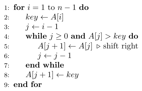
Count the comparisons of the form $A[j] > key$.
$key = 2$: compare with $5$ ($>$, shift). Reached the left end. Array $[2,5,4,6,1,3]$. Comparisons $1$, shifts $1$.
$key = 4$: compare with $5$ (shift), with $2$ (stop). Array $[2,4,5,6,1,3]$. Comparisons $2$, shifts $1$.
$key = 6$: compare with $5$ (stop). Array unchanged. Comparisons $1$, shifts $0$.
$key = 1$: compare with $6,5,4,2$ (all shift), left end reached. Array $[1,2,4,5,6,3]$. Comparisons $4$, shifts $4$.
$key = 3$: compare with $6,5,4$ (shift), with $2$ (stop). Array $[1,2,3,4,5,6]$. Comparisons $4$, shifts $3$.
Total comparisons $= 1+2+1+4+4 = 12$. Total shifts $= 9 = $ inversions of the input.
General formula: shifts $= I$ (number of inversions); comparisons $\le I + (n-1)$. Here $9 + 5 = 14$, minus $2$ because two keys ($2$ and $1$) reached the left end without a failing comparison, giving $12$.
Best case (already sorted): $n-1$ comparisons, $0$ shifts, $\Theta(n)$.
Worst case (reverse sorted): comparisons $=$ shifts $= \dfrac{n(n-1)}{2}$, $\Theta(n^2)$.
Average case: about $\dfrac{n(n-1)}{4}$ inversions, so $\Theta(n^2)$.
Running time $= \Theta(n + I)$, directly proportional to the number of inversions.
Nearly sorted input: if every element is at most $k$ places away from its final position, the time is $O(nk)$.
Stable: yes (we shift only elements strictly greater than the key).
In-place: yes. Adaptive: yes. Online: yes, a new element simply gets inserted into the sorted prefix.
Fastest of the simple sorts for small or nearly sorted arrays; production sorts (TimSort, introsort) use it for small subarrays.
Binary insertion sort: find the insertion position with binary search on the sorted prefix. Comparisons drop to $O(n\log n)$, but the shifting still costs $O(n^2)$ moves, so the total time is still $\Theta(n^2)$. It loses the $\Theta(n)$ best case (it always does about $\log i$ comparisons per key). It remains stable if we search for the position after the last equal element.
Shell sort: insertion sort on elements that are $h$ apart, for a decreasing sequence of gaps $h$, ending with $h=1$. It lets elements jump long distances and beats $\Theta(n^2)$ in practice. Not stable.
Linked-list insertion sort: no shifting is needed (just relink), but finding the position is still linear.
import bisect

def insertion_sort(a):
    comparisons = shifts = 0
    for i in range(1, len(a)):
        key = a[i]
        j = i - 1
        while j >= 0:
            comparisons += 1
            if a[j] > key:
                a[j + 1] = a[j]
                shifts += 1
                j -= 1
            else:
                break
        a[j + 1] = key
    return comparisons, shifts


def binary_insertion_sort(a):
    for i in range(1, len(a)):
        key = a[i]
        pos = bisect.bisect_right(a, key, 0, i)   # after equal elements: stable
        for j in range(i, pos, -1):               # still O(i) shifting
            a[j] = a[j - 1]
        a[pos] = key


A = [5, 2, 4, 6, 1, 3]
print(insertion_sort(A), A)    # (12, 9) [1, 2, 3, 4, 5, 6]
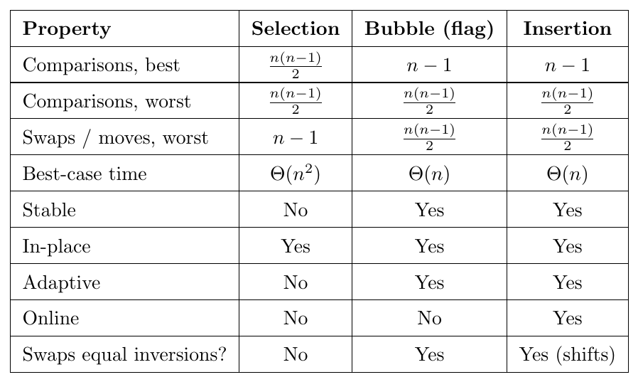
Comparison of the Three Quadratic Sorts
Divide and Conquer Sorting
Merge Sort
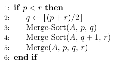
Merge sort follows the divide-and-conquer paradigm:
Divide: split the array into two halves.
Conquer: sort each half recursively (a single element is already sorted).
Combine: merge the two sorted halves into one sorted array.
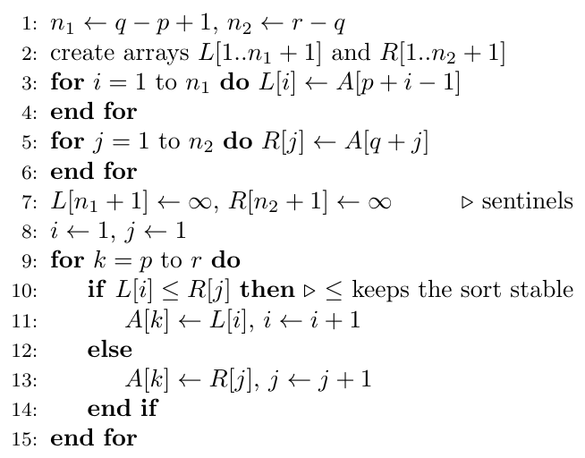
The real work is in the merge step. Merging two sorted lists is easy: keep one pointer at the front of each list, repeatedly take the smaller front element, and move that pointer.
Analogy: Two sorted piles of exam papers (by roll number) on a table. To make one sorted pile, repeatedly compare the top papers of the two piles and take the one with the smaller roll number.
Algorithm: Merge-Sort(A, p, r)
Algorithm: Merge(A, p, q, r) — CLRS style with sentinels
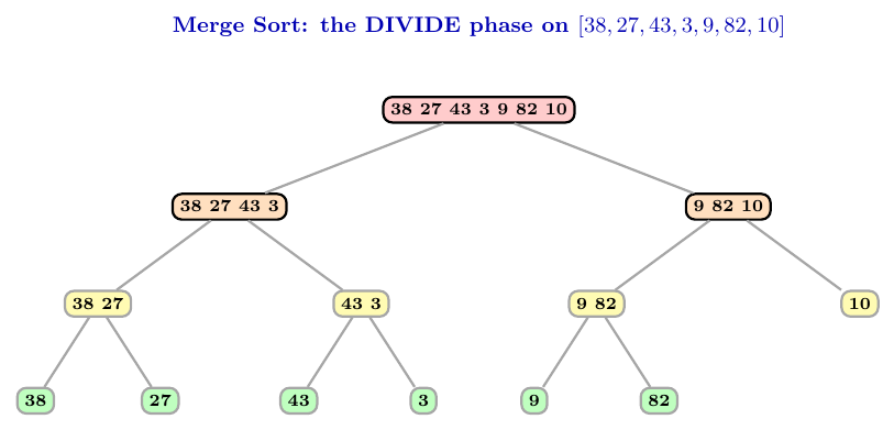
Going up from the leaves:
$[38] + [27] \to [27, 38]$. $[43] + [3] \to [3, 43]$.
$[27, 38] + [3, 43] \to [3, 27, 38, 43]$.
$[9] + [82] \to [9, 82]$. $[9, 82] + [10] \to [9, 10, 82]$.
Final merge: $[3, 27, 38, 43] + [9, 10, 82]$. Compare $3$ vs $9$ (take $3$), $27$ vs $9$ (take $9$), $27$ vs $10$ (take $10$), $27$ vs $82$ (take $27$), $38$ vs $82$ (take $38$), $43$ vs $82$ (take $43$). Left list is empty; copy the remaining $82$ without comparison. Comparisons $= 6$.
Result: $[3, 9, 10, 27, 38, 43, 82]$.
Recurrence: $T(n) = 2T(n/2) + \Theta(n)$. By Master theorem ($a=2$, $b=2$, $n^{\log_2 2} = n = \Theta(f(n))$, Case 2): $T(n) = \Theta(n\log n)$.
By recursion tree: there are $\log_2 n$ levels, and each level does total merge work of about $n$.
Merge comparisons: merging sorted lists of sizes $m$ and $n$ needs
at most $m + n - 1$ comparisons (the largest element ends up in one list and the other list is emptied last);
at least $\min(m, n)$ comparisons (one list entirely smaller than the other).
Comparisons for the whole sort ($n = 2^k$):
Worst case: $n\log_2 n - n + 1$. For $n=8$: $8\cdot 3 - 8 + 1 = 17$.
Best case (already sorted input): $\dfrac{n}{2}\log_2 n$. For $n = 8$: $12$.
Time: $\Theta(n\log n)$ in best, average and worst case. The recurrence does not depend on the input order.
Stable: yes, provided the merge takes from the left list when the elements are equal ($\le$).
Not in-place: needs $\Theta(n)$ auxiliary array for arrays. (Recursion stack adds $O(\log n)$.)
Not adaptive in the basic form (still $\Theta(n\log n)$ on sorted input; only the comparison constant drops).
Not online.
Good for: linked lists (merging needs only $O(1)$ extra space by relinking), external sorting of data larger than memory, and guaranteed $O(n\log n)$.
Bottom-up (iterative) merge sort: merge runs of size $1$, then $2$, then $4$, and so on. No recursion, same $\Theta(n\log n)$.
Natural merge sort: first detect the already-sorted runs in the input and merge those. This is adaptive: $\Theta(n)$ if the input is sorted.
TimSort (used by Python): natural merge sort plus insertion sort for short runs. Stable, adaptive, worst case $\Theta(n\log n)$.
Merge sort on linked lists: $O(1)$ extra space, still stable.
Counting inversions: while merging, whenever an element from the right list is taken before the remaining $x$ elements of the left list, those $x$ pairs are inversions. This counts inversions in $\Theta(n\log n)$ instead of $\Theta(n^2)$.
def merge_sort(a):
    if len(a) <= 1:
        return a
    mid = len(a) // 2
    left = merge_sort(a[:mid])
    right = merge_sort(a[mid:])
    return merge(left, right)


def merge(left, right):
    out = []
    i = j = 0
    while i < len(left) and j < len(right):
        if left[i] <= right[j]:          # <= keeps the sort stable
            out.append(left[i]); i += 1
        else:
            out.append(right[j]); j += 1
    out.extend(left[i:])                 # one of these is empty
    out.extend(right[j:])
    return out


def sort_and_count(a):
    """Returns (sorted list, number of inversions) in O(n log n)."""
    if len(a) <= 1:
        return a, 0
    mid = len(a) // 2
    left, c1 = sort_and_count(a[:mid])
    right, c2 = sort_and_count(a[mid:])
    out, i, j, cross = [], 0, 0, 0
    while i < len(left) and j < len(right):
        if left[i] <= right[j]:
            out.append(left[i]); i += 1
        else:
            out.append(right[j]); j += 1
            cross += len(left) - i       # left[i:] are all > right[j]
    out.extend(left[i:]); out.extend(right[j:])
    return out, c1 + c2 + cross


def bottom_up_merge_sort(a):
    n, width = len(a), 1
    while width < n:
        for lo in range(0, n, 2 * width):
            mid = min(lo + width, n)
            hi = min(lo + 2 * width, n)
            a[lo:hi] = merge(a[lo:mid], a[mid:hi])
        width *= 2


print(merge_sort([38, 27, 43, 3, 9, 82, 10]))
print(sort_and_count([5, 2, 4, 6, 1, 3])[1])     # 9
Quicksort
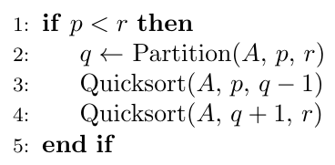
Quicksort also uses divide and conquer, but the hard work is in the divide step (partition), and the combine step is empty.
Divide (partition): choose a pivot and rearrange the array so that elements $\le$ pivot come before it and elements $>$ pivot come after it. The pivot is now in (or near) its final place.
Conquer: sort the left part and the right part recursively.
Combine: nothing to do, since the array is already in order.
Analogy: Arranging a queue by height. Pick one person as the pivot, ask shorter people to stand on his left and taller people on his right, then repeat the idea inside each group.
Algorithm: Quicksort(A, p, r)
Lomuto Partition Scheme (CLRS)
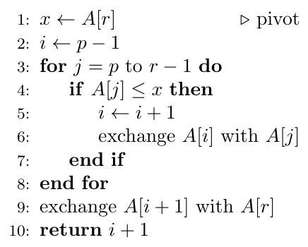
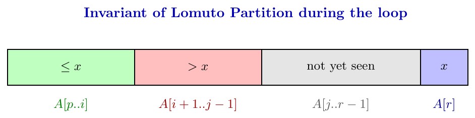
The pivot is the last element $x = A[r]$. We keep an index $i$ such that:
$A[p..i]$ holds elements $\le x$ (the “small” region),
$A[i+1..j-1]$ holds elements $> x$ (the “large” region),
$A[j..r-1]$ is not yet examined.
For each $j$, if $A[j] \le x$, grow the small region by incrementing $i$ and swapping $A[i]$ with $A[j]$. At the end, put the pivot between the two regions by swapping $A[i+1]$ and $A[r]$. The pivot lands at its final sorted position, $i+1$. Partition on $n$ elements does exactly $n-1$ comparisons.
Algorithm: Partition(A, p, r) — Lomuto
Pivot $x = 4$ (last element). $i = -1$ at the start (array indexed from $0$).
$j=0$: $2 \le 4$. $i=0$, swap $A[0]$ with itself. $[2,8,7,1,3,5,6,4]$
$j=1$: $8 > 4$. No change.
$j=2$: $7 > 4$. No change.
$j=3$: $1 \le 4$. $i=1$, swap $A[1]$ and $A[3]$. $[2,1,7,8,3,5,6,4]$
$j=4$: $3 \le 4$. $i=2$, swap $A[2]$ and $A[4]$. $[2,1,3,8,7,5,6,4]$
$j=5$: $5 > 4$. $j=6$: $6 > 4$. No change.
End: swap $A[i+1] = A[3]$ with $A[7]$. $[2,1,3,4,7,5,6,8]$. Pivot index $=3$.
Left part $[2,1,3]$, right part $[7,5,6,8]$. Comparisons in this partition: $7 = n-1$.
Hoare Partition Scheme
The original scheme of C.A.R. Hoare. The pivot is $x = A[p]$ (the first element). Two pointers move towards each other:
$i$ starts at the left and moves right until it finds $A[i] \ge x$.
$j$ starts at the right and moves left until it finds $A[j] \le x$.
If $i < j$, swap $A[i]$ and $A[j]$ and continue. Otherwise return $j$.
The recursion is then on $A[p..j]$ and $A[j+1..r]$. Important differences from Lomuto:
The pivot is not guaranteed to land at its final position.
It does about three times fewer swaps on average, so it is faster in practice.
The recursive calls use $(p, j)$ and $(j+1, r)$, not $(p, q-1)$ and $(q+1, r)$.
With the pivot as the first element and this version, using the last element as pivot can loop forever, so keep the pivot choice and the return value consistent.
Algorithm: Hoare-Partition(A, p, r)
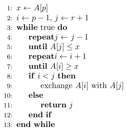
Pivot $x = 5$. Start $i = -1$, $j = 7$.
$j$ moves left: $A[6] = 1 \le 5$, stop at $j=6$. $i$ moves right: $A[0] = 5 \ge 5$, stop at $i=0$. $i<j$, swap: $[1,3,8,4,2,7,5]$.
$j$: $A[5]=7 > 5$, $A[4]=2 \le 5$, stop at $j=4$. $i$: $A[1]=3<5$, $A[2]=8 \ge 5$, stop at $i=2$. Swap: $[1,3,2,4,8,7,5]$.
$j$: $A[3]=4 \le 5$, stop at $j=3$. $i$: $A[3]=4<5$, $A[4]=8\ge5$, stop at $i=4$. Now $i \ge j$, return $j = 3$.
Partitions: $[1,3,2,4]$ and $[8,7,5]$. Every element of the left part is $\le 5 \le$ every element of the right part. Note the pivot $5$ is in the right part, not at a fixed final position.
Analysis of Quicksort
Let the partition split $n$ elements into parts of size $k$ and $n-k-1$ (Lomuto). Then \[ T(n) = T(k) + T(n-k-1) + \Theta(n) \]
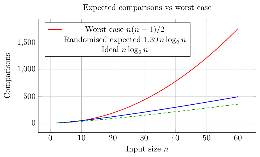
Worst case: the split is always $0 : n-1$ (the pivot is always the smallest or largest element). \[ T(n) = T(n-1) + \Theta(n) \;\Rightarrow\; T(n) = \Theta(n^2), \quad \text{comparisons} = \frac{n(n-1)}{2} \] For $n=5$ this is $4+3+2+1 = 10$ comparisons.
Best case: the pivot is always the median, $T(n) = 2T(n/2) + \Theta(n) = \Theta(n\log n)$.
Any constant-proportion split is still $\Theta(n \log n)$. For example, a $9:1$ split every time gives $T(n) = T(9n/10) + T(n/10) + n$. The recursion tree has depth about $\log_{10/9} n$ on the long side, and each level costs at most $n$, so $T(n) = \Theta(n\log n)$. This is why quicksort is good even with an “unlucky but not terrible” pivot.
Average case: for a random input order, $E[C_n] = (n-1) + \dfrac{2}{n}\sum_{k=0}^{n-1} E[C_k]$, which solves to $\approx 2n\ln n \approx 1.39\, n\log_2 n$ comparisons. So the average is $\Theta(n\log n)$, only about $39\%$ more comparisons than the ideal.
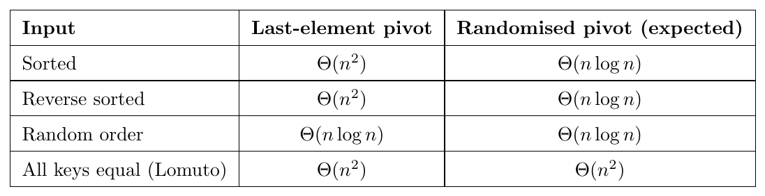
Sorted or reverse-sorted input with first or last element as pivot: every partition is $0 : n-1$, so $\Theta(n^2)$. (Sorted + last-element pivot: the pivot is the maximum. Reverse sorted + last-element pivot: the pivot is the minimum.)
All elements equal with Lomuto's “$\le$” test: every element goes to the left part, so the split is again $n-1 : 0$ and the time is $\Theta(n^2)$.
Middle element as pivot makes sorted input the best case, but an adversary can still construct a bad input for any fixed pivot rule.
Pivot is always the median (found in $O(n)$ time) gives a guaranteed $\Theta(n\log n)$ worst case, but with a big constant.
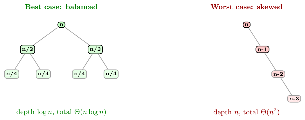
Time: best and average $\Theta(n\log n)$, worst $\Theta(n^2)$.
In-place: yes, partitioning rearranges within the array. The recursion stack uses $O(\log n)$ on average, but $O(n)$ in the worst case.
Not stable: the long-distance swaps in partition can reorder equal elements. Example with Lomuto on $[3_a, 3_b, 2]$: pivot $2$; no element is $\le 2$ except the pivot itself, and the final swap gives $[2, 3_b, 3_a]$. The two $3$s are reversed.
Not adaptive in the basic form, and not online.
Fast in practice: good cache behaviour (sequential access) and a small constant factor, usually faster than merge sort on arrays.
Randomised quicksort: choose the pivot uniformly at random (or swap a random element to the pivot position first). No fixed input is bad; for every input the expected time is $O(n\log n)$. The worst case $O(n^2)$ still exists but has negligible probability.
Median-of-three pivot: use the median of the first, middle and last elements. Sorted input is handled well.
Three-way partitioning (Dutch national flag): split into $<$ pivot, $=$ pivot, $>$ pivot. Equal elements are placed once and never touched again, so inputs with many duplicates run in $O(n)$ for all-equal input.
Smaller-part-first recursion + tail-call elimination: recurse on the smaller side and loop on the larger side. The stack depth is at most $\log_2 n$, so the stack space is $O(\log n)$ even in the worst case.
Introsort: start with quicksort; if the recursion depth exceeds $2\log_2 n$, switch to heap sort. Guarantees $O(n\log n)$ worst case. Used in C++
std::sort.Cutoff to insertion sort for tiny subarrays (below about $10$ elements).
Partition(A, p, r):
x = A[r], i = p - 1
for j = p to r - 1:
if A[j] $<=$ x: i = i + 1, swap(A[i], A[j])
swap(A[i+1], A[r])
return i + 1
Quicksort(A, p, r):
if p < r:
q = Partition(A, p, r)
Quicksort(A, p, q - 1)
Quicksort(A, q + 1, r)
import random

def lomuto_partition(a, p, r):
    x = a[r]
    i = p - 1
    for j in range(p, r):
        if a[j] <= x:
            i += 1
            a[i], a[j] = a[j], a[i]
    a[i + 1], a[r] = a[r], a[i + 1]
    return i + 1


def quicksort(a, p, r):
    if p < r:
        q = lomuto_partition(a, p, r)
        quicksort(a, p, q - 1)
        quicksort(a, q + 1, r)


def hoare_partition(a, p, r):
    x = a[p]
    i, j = p - 1, r + 1
    while True:
        j -= 1
        while a[j] > x:
            j -= 1
        i += 1
        while a[i] < x:
            i += 1
        if i < j:
            a[i], a[j] = a[j], a[i]
        else:
            return j


def quicksort_hoare(a, p, r):
    if p < r:
        q = hoare_partition(a, p, r)
        quicksort_hoare(a, p, q)          # note: q, not q-1
        quicksort_hoare(a, q + 1, r)


def randomized_quicksort(a, p, r):
    if p < r:
        k = random.randint(p, r)
        a[k], a[r] = a[r], a[k]           # random pivot moved to the end
        q = lomuto_partition(a, p, r)
        randomized_quicksort(a, p, q - 1)
        randomized_quicksort(a, q + 1, r)


def three_way_quicksort(a, lo, hi):
    """Dutch national flag partition: handles duplicates well."""
    if lo >= hi:
        return
    x = a[lo]
    lt, i, gt = lo, lo + 1, hi
    while i <= gt:
        if a[i] < x:
            a[lt], a[i] = a[i], a[lt]; lt += 1; i += 1
        elif a[i] > x:
            a[i], a[gt] = a[gt], a[i]; gt -= 1
        else:
            i += 1
    three_way_quicksort(a, lo, lt - 1)
    three_way_quicksort(a, gt + 1, hi)


A = [2, 8, 7, 1, 3, 5, 6, 4]
print(lomuto_partition(A[:], 0, 7), A)       # pivot index 3
B = [2, 8, 7, 1, 3, 5, 6, 4]
quicksort(B, 0, len(B) - 1)
print(B)                                      # [1, 2, 3, 4, 5, 6, 7, 8]
Lower Bound for Comparison-Based Sorting
A comparison-based sorting algorithm can be viewed as a binary decision tree. Each internal node is a comparison “is $a_i < a_j$?”, and each leaf is one possible output ordering (a permutation of the input).
There are $n!$ possible input orderings, and the algorithm must be able to produce each of them, so the tree has at least $n!$ leaves.
A binary tree of height $h$ has at most $2^h$ leaves. So $2^h \ge n!$, which gives \[ h \ge \log_2(n!) \]
The height $h$ is the number of comparisons in the worst case. Using Stirling's approximation, $\log_2 (n!) = n\log_2 n - n\log_2 e + O(\log n) = \Theta(n\log n)$.
Hence every comparison sort needs $\Omega(n\log n)$ comparisons in the worst case. This proves that merge sort (and heap sort) are asymptotically optimal.
Minimum worst-case comparisons to sort $n$ elements is at least $\lceil \log_2 n! \rceil$: for $n=3$, $\lceil\log_2 6\rceil = 3$; for $n=4$, $\lceil\log_2 24\rceil = 5$; for $n=5$, $\lceil\log_2 120\rceil = 7$.
Searching a sorted array: the decision tree for a key among $n$ sorted elements has $n$ successful outcomes, so the height is at least $\lceil\log_2(n+1)\rceil$. Binary search meets this bound.
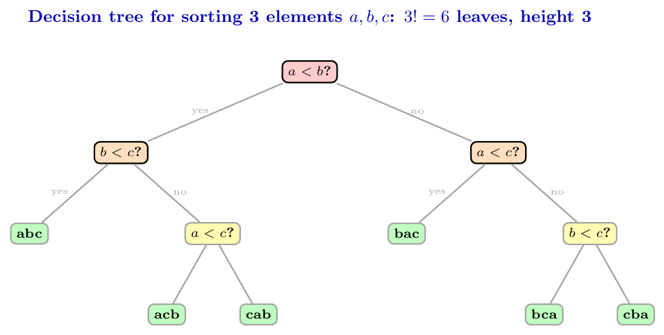
Can we sort $6$ numbers using only $9$ comparisons in the worst case? $6! = 720$ and $2^9 = 512 < 720$. A decision tree with $9$ levels has at most $512$ leaves, which is less than $720$, so it is impossible. We need at least $\lceil \log_2 720 \rceil = 10$ comparisons.
Randomised Quicksort
In ordinary quicksort the pivot rule is fixed (first, last or middle element). So for every fixed rule there is some input, such as a sorted array, that gives $\Theta(n^2)$ time. A person who knows your rule can always give you that bad input.
In randomised quicksort, the pivot is chosen uniformly at random from the current subarray. Now the running time depends on the coin tosses of the algorithm and not on the order of the input. No input is bad in itself. For every input, the expected running time is $\Theta(n\log n)$.
Analogy: A teacher picks a student at random as the “pivot” for splitting the class by height. Because the student is picked by lottery, nobody can arrange the class in advance to make the teacher unlucky.
Algorithm: Randomized-Partition(A, p, r)

Algorithm: Randomized-Quicksort(A, p, r)
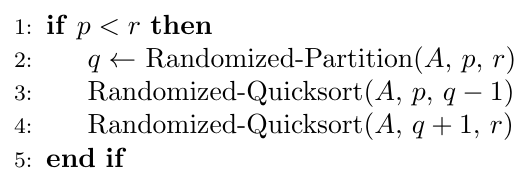
RandomizedPartition(A, p, r):
i = random integer in [p, r]
swap(A[r], A[i])
return Partition(A, p, r)
RandomizedQuicksort(A, p, r):
if p < r:
q = RandomizedPartition(A, p, r)
RandomizedQuicksort(A, p, q - 1)
RandomizedQuicksort(A, q + 1, r)
Examples
Sort $A = [1, 2, 3, 4, 5]$, which is the worst input for last-element pivot.
Call 1: the random index chosen is $2$ (value $3$). Swap with $A[4]$: $[1,2,5,4,3]$. Lomuto with pivot $3$: elements $1, 2$ are $\le 3$, elements $5, 4$ are not. Final swap gives $[1,2,3,4,5]$ with pivot index $2$. Split sizes $2 : 2$. Comparisons: $4$.
Left part $[1,2]$: random pivot, say index $0$. Swap: $[2,1]$. Pivot $1$: $2 > 1$. Final swap gives $[1,2]$. Comparisons: $1$. Right part $[4,5]$ similarly costs $1$ comparison.
Total comparisons $= 4 + 1 + 1 = 6$, instead of the $10$ that last-element pivot needs on this input.
For $n = 3$ distinct elements, the first pivot is the smallest, the middle or the largest, each with probability $\tfrac13$.
Pivot is the middle element (probability $\tfrac13$): the split is $1:1$. Comparisons $= 2$ (partition) $+ 0 + 0 = 2$.
Pivot is the smallest or largest (probability $\tfrac23$): the split is $0:2$. Comparisons $= 2$ (partition) $+ 1$ (sorting two elements) $= 3$.
Expected comparisons $= \tfrac13(2) + \tfrac23(3) = \tfrac83 \approx 2.67$.
For $n = 4$, the maximum number of comparisons is $3 + 2 + 1 = 6$. This happens when every pivot is the minimum or maximum of its subarray. The first call has $2$ good choices out of $4$, the second has $2$ out of $3$, the third has $2$ out of $2$. \[ \Pr[\text{6 comparisons}] = \frac24 \cdot \frac23 \cdot \frac22 = \frac13 \] In general, the probability of the fully skewed run is $\dfrac{2^{n-1}}{n!}$. For $n = 10$ this is $\dfrac{512}{3628800} \approx 0.00014$, and it falls extremely fast as $n$ grows.
Sort $6$ distinct elements. What is the probability that the elements of rank $2$ and rank $5$ are ever compared?
They are compared only if one of them is the first pivot chosen among the ranks $2,3,4,5$. If any element of rank $3$ or $4$ is chosen first, it separates them forever. There are $5 - 2 + 1 = 4$ elements in the range, and $2$ of them are good choices. \[ \Pr = \frac{2}{4} = \frac12 \]
Performance
import random

comparisons = 0

def partition(a, p, r):
    global comparisons
    x = a[r]
    i = p - 1
    for j in range(p, r):
        comparisons += 1
        if a[j] <= x:
            i += 1
            a[i], a[j] = a[j], a[i]
    a[i + 1], a[r] = a[r], a[i + 1]
    return i + 1


def randomized_partition(a, p, r):
    i = random.randint(p, r)          # uniform in [p, r]
    a[r], a[i] = a[i], a[r]
    return partition(a, p, r)


def randomized_quicksort(a, p, r):
    while p < r:                      # loop on the larger part
        q = randomized_partition(a, p, r)
        if q - p < r - q:             # recurse on the smaller part
            randomized_quicksort(a, p, q - 1)
            p = q + 1
        else:
            randomized_quicksort(a, q + 1, r)
            r = q - 1


def average_comparisons(n, trials=2000):
    global comparisons
    total = 0
    for _ in range(trials):
        a = list(range(n))            # sorted input: worst for fixed pivot
        comparisons = 0
        randomized_quicksort(a, 0, n - 1)
        total += comparisons
    return total / trials


for n in (3, 10, 100, 1000):
    print(n, round(average_comparisons(n), 1))
# n=3    ~ 2.67
# n=100  ~ 648    (formula 2(n+1)H(n+1) - 4n)
# n=1000 ~ 10987
Master Summary
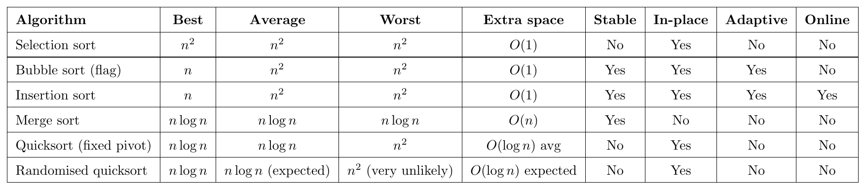
Count the right thing. Some questions ask comparisons, some ask swaps, some ask passes. Selection sort: comparisons fixed at $\frac{n(n-1)}{2}$. Bubble and insertion: swaps (shifts) $=$ number of inversions.
Stability traps. Stable: bubble, insertion, merge. Not stable: selection, quicksort (and heap sort). Selection sort can be made stable by shifting; merge sort becomes unstable if the merge uses $<$ instead of $\le$.
Quicksort worst case. Sorted or reverse-sorted input with first or last pivot, and also all-equal elements with Lomuto. Recurrence $T(n)=T(n-1)+n$. A constant split ratio (like $9:1$) is still $\Theta(n \log n)$.
Randomised quicksort. Expected time is $O(n\log n)$ for every input, worst case is still $O(n^2)$. Probability that ranks $i<j$ are compared is $\frac{2}{j-i+1}$.
In-place is not the same as no extra stack. Quicksort is in-place (it needs only $O(\log n)$ stack on average). Merge sort on arrays is not in-place.
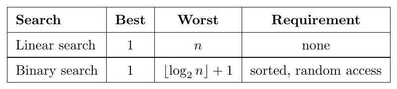
Binary search iterations for $n$ elements: at most $\lfloor\log_2 n\rfloor + 1$. Do not forget the $+1$.
Lower bound. For $n!$ outcomes, at least $\lceil\log_2 n!\rceil$ comparisons.
Quicksort partition trace. Know the Lomuto scheme (pivot last) and the Hoare scheme (pivot first, pointers towards each other) by hand. They give different intermediate arrays.