Graph Traversals
Graph traversal means visiting every vertex of a graph in a systematic way, making sure no vertex is missed and no vertex is visited twice. Unlike arrays or linked lists where there is only one natural order to visit elements, a graph can be traversed in many different ways depending on the strategy used. The two most fundamental and important traversal strategies are Breadth-First Search (BFS) and Depth-First Search (DFS).
Traversal is the foundation for solving many graph problems: finding shortest paths, detecting cycles, topological sorting, finding connected components, and many more. Mastering BFS and DFS step-by-step tracing is the single highest-yield graph topic in competitive exams.
Breadth-First Search (BFS)
Introduction to BFS
Breadth-First Search (BFS) explores a graph level by level, outward from a chosen source vertex. It visits all neighbours of the current vertex before moving any deeper into the graph. BFS uses a FIFO queue to control the order of traversal, which is exactly what guarantees the level-by-level behaviour.
Finding the shortest path (fewest edges) in an unweighted graph.
Finding all connected components of a graph.
Level-order traversal of a tree (BFS applied to a tree is exactly level-order traversal).
BFS Algorithm
Each vertex is given a color to track its traversal state:
WHITE: not yet discovered.
GRAY: discovered, but still has unexplored neighbours (currently in the queue).
BLACK: fully explored, all its neighbours have been looked at.
Along with color, we track $d[v]$ (distance from source $s$) and $\pi[v]$ (the parent of $v$ in the BFS tree).
Algorithm: BFS(G, s)
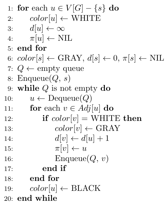
With an adjacency list, each vertex is enqueued and dequeued exactly once ($O(V)$ total), and each edge is examined at most twice across the whole run ($O(E)$ total). So BFS runs in $O(V + E)$ time. With an adjacency matrix, finding the neighbours of a vertex takes $O(V)$ each time, giving $O(V^2)$ total.
BFS Trace: Example Graph
Consider the undirected graph with vertices $\{A, B, C, D, E\}$ and edges $\{(A,B), (A,C), (B,C), (C,D), (C,E)\}$. Adjacency lists (alphabetical order): $A:[B,C]$, $B:[A,C]$, $C:[A,B,D,E]$, $D:[C]$, $E:[C]$. BFS starts from source $A$.
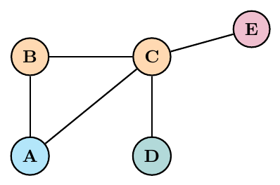
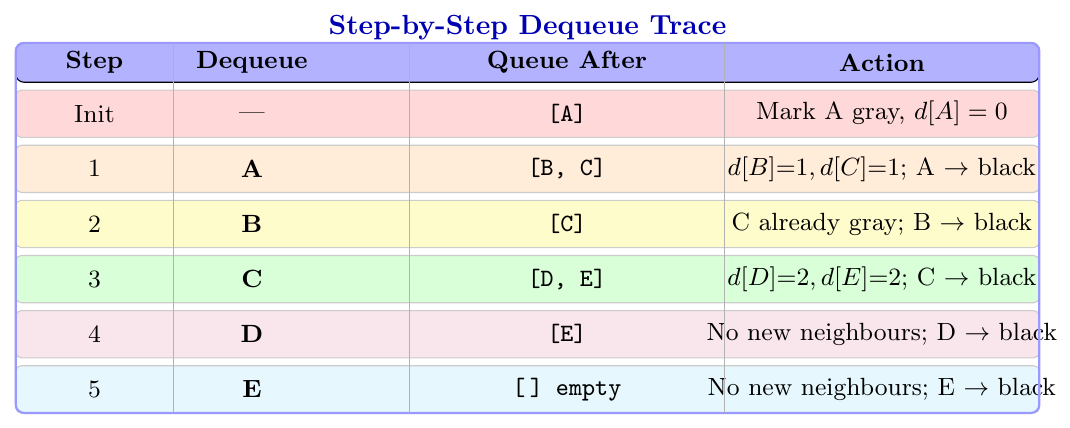
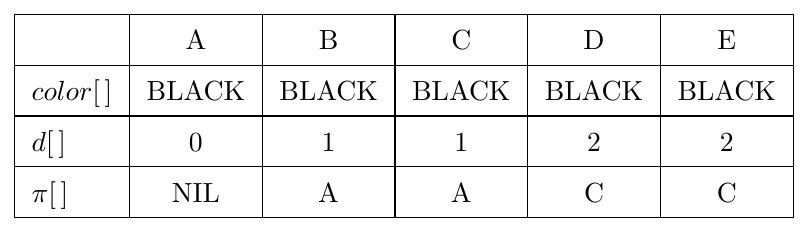
BFS order (dequeue order): $A, B, C, D, E$
BFS on Directed Graphs
The core logic and the $O(V+E)$ complexity are identical for directed graphs. BFS simply follows the outbound edges listed in $Adj[u]$; it never looks at incoming edges.
Take the same 5 vertices, but now the edges are directed: $A\to B$, $A\to C$, $B\to C$, $C\to D$, $C\to E$. BFS from source $A$.
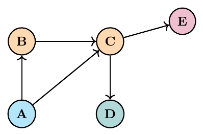
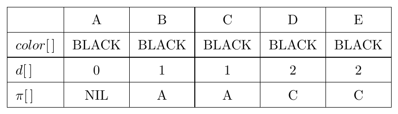
Since $B$'s only out-neighbour $C$ is already discovered (via $A$) by the time $B$ is processed, the resulting distances and parents come out exactly the same as the undirected case here.
BFS on Disconnected Graph — Connected Components
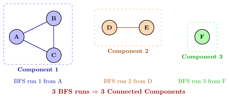
If the graph is disconnected, a single BFS from one source will not reach all vertices. To find all connected components, we run BFS from every unvisited vertex. Each BFS run that starts fresh (from an unvisited vertex) discovers one complete connected component.
The number of times we start BFS from an unvisited source = the number of connected components.
Properties of BFS
Multiple valid BFS orderings can exist for the same graph, depending on:
which vertex is chosen as the source,
the order in which neighbours appear in the adjacency list.
Changing either of these can give a different but equally valid BFS sequence.
$d[u]$ equals the exact level of $u$ in the BFS tree. In our example graph: $d[A] = 0$ (Level 0), $d[B] = d[C] = 1$ (Level 1), $d[D] = d[E] = 2$ (Level 2).
The sequence in which vertices are removed from the queue (DEQUEUE calls) is the BFS traversal order. For our example: \[ A, B, C, D, E \]
In an unweighted graph, $d[u]$ gives the minimum number of edges on any path from $s$ to $u$. In our example, $d[D] = 2$ means the shortest path from $A$ to $D$ uses exactly 2 edges: $A \to C \to D$.
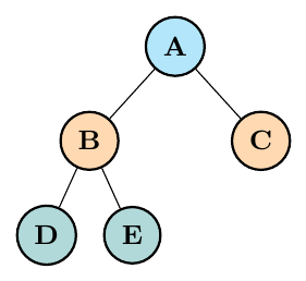
BFS applied to a tree is exactly the same thing as level-order traversal. No cycle detection or visited array is even needed, because a tree has no cycles, so a vertex can never be reached a second time.
Run BFS from any unvisited (WHITE) vertex. Each full BFS call discovers exactly one entire connected component. Repeating this until every vertex has been visited, and counting how many times BFS was started, gives the total number of connected components.
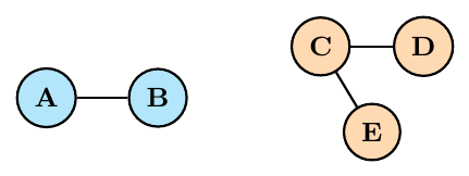
2 calls to BFS are needed to cover every vertex here, so the graph has 2 connected components: $\{A, B\}$ and $\{C, D, E\}$.
A tree edge is an edge $(u,v)$ that first discovers a new WHITE vertex $v$. The collection of all tree edges forms the BFS spanning tree.
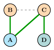
In this graph, the solid green edges $(A,B)$, $(A,C)$, $(C,D)$ are tree edges, since each one first discovers a new vertex. The dashed edge $(B,C)$ connects two vertices that are both already discovered, so it is not a tree edge.
A cross edge is a non-tree edge connecting two vertices that are both already discovered. In an undirected BFS tree, a cross edge always satisfies: \[ |d[u] - d[v]| \le 1 \]
Edge $(B, C)$ from the previous diagram is a cross edge. Here $d[B] = 1$ and $d[C] = 1$, so $|d[B] - d[C]| = 0 \le 1$, which confirms it is a valid cross edge.
A back edge is a directed edge from a descendant back to an ancestor in the BFS tree. Back edges can only occur in directed graphs that contain a cycle; they never occur in an undirected BFS tree.
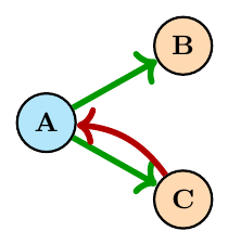
Edge $(C, A)$ (red, directed back to the root) is a back edge. This situation cannot happen in an undirected BFS tree, because if $A \to C$ exists, then $(A,C)$ already becomes a tree edge the moment $C$ is first discovered, which would make $C \to A$ redundant rather than a separate back edge.
A forward edge would be a hypothetical edge from an ancestor to a non-child descendant further down the tree. Such edges never appear in any BFS tree, directed or undirected.
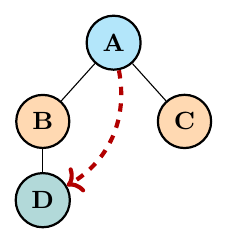
BFS always discovers the shallowest reachable vertices first. If an edge $A \to D$ really existed, then $D$ would have been discovered directly from $A$ at Level 1, not through $B$ at Level 2. So this hypothetical dashed edge (a "forward edge") is a contradiction, and it simply cannot occur in a BFS tree.
The maximum size the queue ever reaches during BFS equals the widest level of the BFS tree: \[ \text{Max Queue Size} = \max_{k} \left| \{v \in V : d[v] = k\} \right| \]
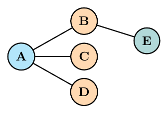
Level 1 contains 3 vertices ($B$, $C$, $D$), which is the widest level in this graph (Level 0 has only $A$, Level 2 has only $E$). So the maximum queue size reached during this BFS run is $\boxed{3}$.
At any point during BFS, if the queue contains $Q = \langle v_1, v_2, \ldots, v_r \rangle$ (front to back), then: \[ d[v_1] \le d[v_2] \le \cdots \le d[v_r], \qquad d[v_r] - d[v_1] \le 1 \] In other words, the queue is always sorted by distance, and it never spans more than two consecutive levels at once. You can never have two vertices whose distances differ by 2 or more sitting in the queue at the same time.
If, while running BFS, we find an edge $(u,v)$ such that \[ d[u] \equiv d[v] \pmod{2} \] (both distances have the same parity), then the graph contains an odd-length cycle.
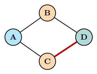
Here $d[C] = 1$ and $d[D] = 1$ (discovered via $B$). The edge $(C,D)$, shown in red, connects two vertices at the same distance (both odd). By the rule, this forces an odd cycle to exist: following $A \to B \to D \to C \to A$ traces out a cycle of length 4 through the tree plus this cross edge; more precisely, the presence of an edge joining two same-parity levels is what certifies an odd cycle exists somewhere in the graph.
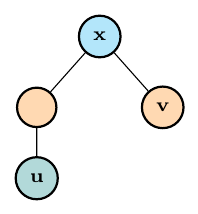
To find the diameter of a tree (the length of the longest path between any two vertices), we do not need to try all pairs. A clever shortcut works:
Run BFS from any arbitrary vertex $x$. Find the vertex $u$ that is farthest from $x$.
Run BFS again, this time from $u$. Find the vertex $v$ that is farthest from $u$.
The distance $d[v]$ found in the second BFS pass is exactly the diameter of the tree.
While BFS explores neighbour $v$ of the current vertex $u$: if $v$ is already visited AND $v \ne \pi[u]$ (i.e., $v$ is not the parent of $u$), then a cycle has been detected.
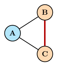
BFS from $A$: visit $B$, set $\pi[B] = A$. Visit $C$, set $\pi[C] = A$. When $B$ later checks its neighbour $C$ (the red edge), $C$ is already visited, and $C \ne \pi[B] = A$. This confirms a cycle exists: $A$–$B$–$C$–$A$.
from collections import deque

WHITE, GRAY, BLACK = 0, 1, 2

def bfs(graph, s, vertices):
    color = {v: WHITE for v in vertices}
    d     = {v: float('inf') for v in vertices}
    pi    = {v: None for v in vertices}

    color[s] = GRAY
    d[s]     = 0
    order    = []

    Q = deque([s])
    while Q:
        u = Q.popleft()
        order.append(u)
        for v in graph[u]:
            if color[v] == WHITE:
                color[v] = GRAY
                d[v]     = d[u] + 1
                pi[v]    = u
                Q.append(v)
        color[u] = BLACK

    return order, d, pi


def count_components(graph, vertices):
    visited = {v: False for v in vertices}
    count   = 0
    for v in vertices:
        if not visited[v]:
            count += 1
            Q = deque([v])
            visited[v] = True
            while Q:
                u = Q.popleft()
                for w in graph[u]:
                    if not visited[w]:
                        visited[w] = True
                        Q.append(w)
    return count


def tree_diameter(graph, vertices):
    """Two-pass BFS to find the diameter of a tree."""
    _, d1, _ = bfs(graph, vertices[0], vertices)
    u = max(d1, key=d1.get)          # farthest vertex from arbitrary start
    _, d2, _ = bfs(graph, u, vertices)
    v = max(d2, key=d2.get)          # farthest vertex from u
    return d2[v]                      # diameter


# --- Driver Code ---
vertices = ['A', 'B', 'C', 'D', 'E']
graph = {
    'A': ['B', 'C'],
    'B': ['A', 'C'],
    'C': ['A', 'B', 'D', 'E'],
    'D': ['C'],
    'E': ['C'],
}

order, d, pi = bfs(graph, 'A', vertices)
print("BFS order:", order)   # ['A', 'B', 'C', 'D', 'E']
print("Distances:", d)       # {'A':0,'B':1,'C':1,'D':2,'E':2}
print("Parents:", pi)        # {'A':None,'B':'A','C':'A','D':'C','E':'C'}
Depth-First Search (DFS)
DFS explores a graph by going as deep as possible along each path before backtracking. Starting from a source vertex, it visits one neighbour, then one of that neighbour's neighbours, and keeps going deeper until it reaches a vertex with no unvisited neighbours. Then it backtracks and tries another direction.
DFS uses a stack (or recursion, which uses the call stack implicitly). Think of exploring a maze by always taking the first available turn, going as far as you can, then backing up when you hit a dead end.
Imagine exploring a cave with many tunnels branching off. You always take the first unexplored tunnel and go as deep as possible. When you hit a dead end, you back up to the last junction and take the next unexplored tunnel. DFS works exactly this way.
DFS Discovery and Finish Timestamps
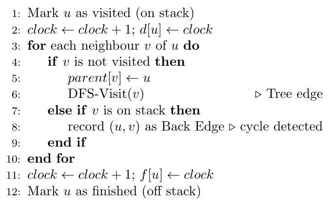
In DFS, we maintain a global counter (clock). Two timestamps are recorded for each vertex $v$:
Discovery time $d[v]$: the clock value when $v$ is first visited (entered).
Finish time $f[v]$: the clock value when DFS has finished exploring all of $v$'s descendants (exited).
For any vertex $v$, $d[v] < f[v]$. If $u$ is an ancestor of $v$ in the DFS tree, then $d[u] < d[v] < f[v] < f[u]$, meaning the interval $[d[v], f[v]]$ is completely inside $[d[u], f[u]]$.
This parenthesis theorem is very important for classifying edges.
DFS Step-by-Step Trace with Timestamps
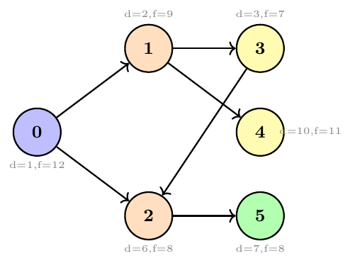
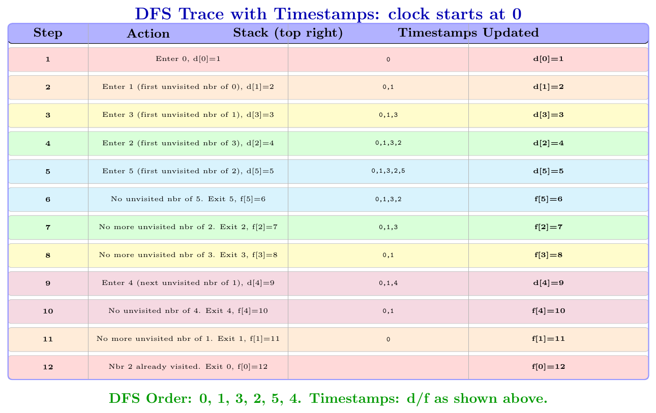
Graph with 6 vertices, edges: $0\to1, 0\to2, 1\to3, 1\to4, 2\to5, 3\to2$. Start from vertex 0. Neighbours visited in increasing order.
DFS Edge Classification
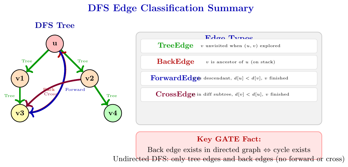
During DFS on a directed graph, every edge $(u, v)$ falls into exactly one of four categories:
Tree Edge: $(u, v)$ is a tree edge if $v$ was discovered for the first time through $u$. It is the edge used to discover a new vertex. It appears in the DFS tree.
Back Edge: $(u, v)$ is a back edge if $v$ is an ancestor of $u$ in the DFS tree (i.e., $v$ is still on the recursion stack when we see this edge). Back edges indicate a cycle in a directed graph.
Forward Edge: $(u, v)$ is a forward edge if $v$ is a descendant of $u$ in the DFS tree, but $v$ was not discovered directly through $u$ (it was discovered through some other path). Identified by $d[u] < d[v]$ and $v$ already finished.
Cross Edge: $(u, v)$ is a cross edge if $v$ is in a different DFS subtree (not an ancestor or descendant of $u$). Identified by $d[v] < d[u]$ and $v$ already finished.
When DFS is exploring vertex $u$ and encounters edge $(u, v)$:
If $v$ is unvisited: Tree Edge.
If $v$ is currently on the DFS stack (visited but not finished): Back Edge.
If $v$ is already finished and $d[u] < d[v]$: Forward Edge.
If $v$ is already finished and $d[u] > d[v]$: Cross Edge.
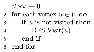
Algorithm: DFS(G)
Algorithm: DFS-Visit(u)
def dfs_full(graph, n):
    visited  = [False] * n
    on_stack = [False] * n   # currently in recursion stack
    d        = [0] * n       # discovery time
    f        = [0] * n       # finish time
    parent   = [-1] * n
    clock    = [0]           # use list so nested function can modify it
    order    = []
    has_cycle = [False]

    def dfs_visit(u):
        visited[u]  = True
        on_stack[u] = True
        clock[0]   += 1
        d[u]        = clock[0]
        order.append(u)

        for v in graph[u]:
            if not visited[v]:
                parent[v] = u
                dfs_visit(v)
            elif on_stack[v]:
                has_cycle[0] = True   # back edge = cycle

        clock[0]   += 1
        f[u]        = clock[0]
        on_stack[u] = False

    for i in range(n):
        if not visited[i]:
            dfs_visit(i)

    return order, d, f, parent, has_cycle[0]


# --- Driver Code ---
# Directed graph: 0->1, 0->2, 1->3, 1->4, 2->5, 3->2
n     = 6
graph = {0:[1,2], 1:[3,4], 2:[5], 3:[2], 4:[], 5:[]}

order, d, f, parent, cycle = dfs_full(graph, n)
print("DFS order:", order)
print("Discovery:", d)
print("Finish:   ", f)
print("Has cycle:", cycle)

# Output:
# DFS order: [0, 1, 3, 2, 5, 4]
# Discovery: [1, 2, 4, 3, 9, 5]
# Finish:    [12, 11, 8, 8, 10, 6]
# Has cycle: False
Topological Sort
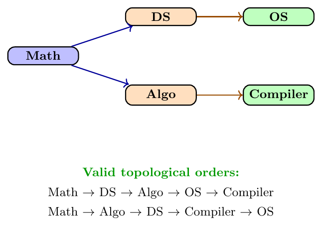
A topological sort (or topological ordering) of a DAG (Directed Acyclic Graph) is a linear ordering of all its vertices such that for every directed edge $(u, v)$, vertex $u$ appears before vertex $v$ in the ordering.
Think of scheduling tasks where some tasks must be completed before others. For example, you must wear socks before shoes, wear shirt before jacket. A topological sort gives a valid sequence of completing all tasks.
Topological sort is only defined for DAGs. If the graph has a cycle, no topological ordering exists.
Suppose courses have prerequisites: Math before DS, Math before Algo, DS before OS, Algo before Compiler. A topological sort gives a valid order to take these courses without violating any prerequisite.
Method 1: DFS-Based Topological Sort
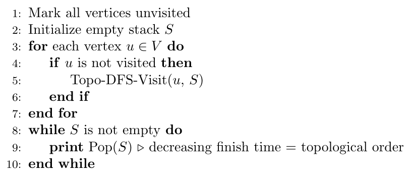
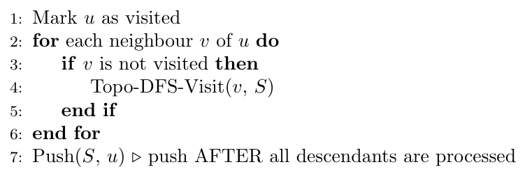
When DFS finishes a vertex $u$ (assigns finish time), we push $u$ onto a stack. After DFS completes for all vertices, we pop the stack to get the topological order. The vertex with the largest finish time comes first in the topological order.
Why it works: If there is an edge $(u, v)$, then DFS on $u$ must complete all of $v$'s work before $u$ finishes. So $f[v] < f[u]$, meaning $u$ finishes after $v$, so $u$ appears before $v$ when we output in decreasing finish time order.
Graph: $0 \to 1, 0 \to 2, 1 \to 3, 2 \to 3$. This is a DAG.
DFS from 0: discover 0, then 1, then 3. Finish 3 (push 3). Back to 1, finish 1 (push 1). Back to 0, go to 2, discover 2. Finish 2 (wait, 3 already finished). Finish 2 (push 2). Finish 0 (push 0).
Stack (top to bottom): 0, 2, 1, 3. Pop gives: 0, 2, 1, 3.
Verify: edge $0\to1$: 0 before 1 $\checkmark$, edge $0\to2$: 0 before 2 $\checkmark$, edge $1\to3$: 1 before 3 $\checkmark$, edge $2\to3$: 2 before 3 $\checkmark$.
Algorithm: Topological-Sort-DFS(G)
Algorithm: Topo-DFS-Visit(u, S)
Method 2: Kahn's Algorithm (BFS with In-Degree)
Kahn's algorithm is an iterative BFS-based method. The key insight is: in a topological ordering, the first vertex must have in-degree 0 (no prerequisites). After removing it, the next vertex with in-degree 0 can come next, and so on.
Steps:
Compute the in-degree of every vertex.
Add all vertices with in-degree 0 to a queue.
While the queue is not empty:
Dequeue vertex $u$, add it to the topological order.
For each neighbour $v$ of $u$: decrease $v$'s in-degree by 1. If $v$'s in-degree becomes 0, enqueue $v$.
If the topological order contains fewer than $|V|$ vertices, the graph has a cycle.
This also detects cycles: if we cannot empty the queue before visiting all vertices, a cycle exists.
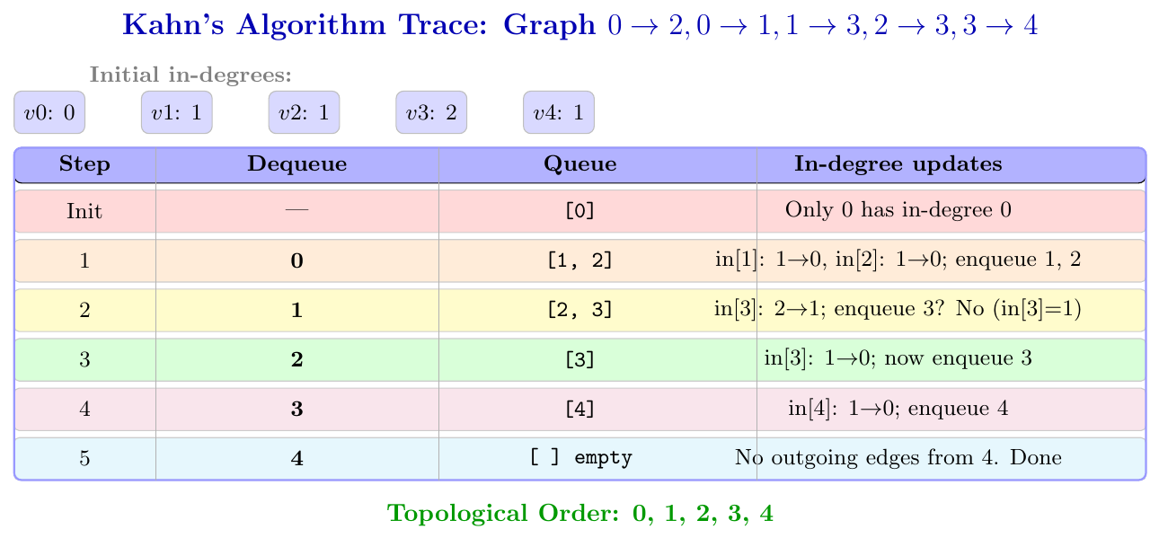
Algorithm: Kahn-Topological-Sort(G)
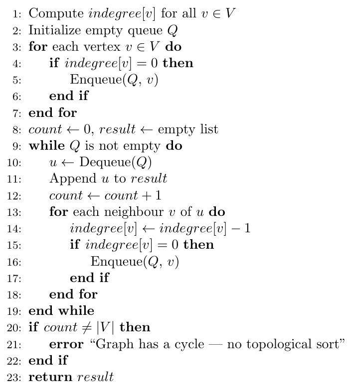
A DAG may have many valid topological orderings. The order in which we add zero-in-degree vertices to the queue (and which queue we use) determines the specific ordering produced. For the graph $0\to2, 0\to1, 1\to3, 2\to3$:
If we process 1 before 2 at step 2: order is 0, 1, 2, 3.
If we process 2 before 1 at step 2: order is 0, 2, 1, 3.
Both are valid. The DAG does not have a unique topological ordering unless it is a Hamiltonian path (each vertex has at most one zero-in-degree vertex at any time during Kahn's).
from collections import deque

# ============================================================
# Method 1: DFS-Based Topological Sort
# ============================================================
def topo_sort_dfs(graph, n):
    visited = [False] * n
    stack   = []

    def dfs_visit(u):
        visited[u] = True
        for v in graph[u]:
            if not visited[v]:
                dfs_visit(v)
        stack.append(u)   # push AFTER all descendants

    for i in range(n):
        if not visited[i]:
            dfs_visit(i)

    return stack[::-1]   # reverse = topological order


# ============================================================
# Method 2: Kahn's Algorithm (BFS with in-degree)
# ============================================================
def kahn_topo_sort(graph, n):
    indegree = [0] * n
    for u in range(n):
        for v in graph[u]:
            indegree[v] += 1

    queue = deque()
    for v in range(n):
        if indegree[v] == 0:
            queue.append(v)

    result = []
    while queue:
        u = queue.popleft()
        result.append(u)
        for v in graph[u]:
            indegree[v] -= 1
            if indegree[v] == 0:
                queue.append(v)

    if len(result) != n:
        print("Cycle detected! No topological sort possible.")
        return []
    return result


# --- Driver Code ---
# DAG: 0->2, 0->1, 1->3, 2->3, 3->4
n     = 5
graph = {0:[1,2], 1:[3], 2:[3], 3:[4], 4:[]}

print("DFS Topo Sort:", topo_sort_dfs(graph, n))
# Output: [0, 2, 1, 3, 4] or [0, 1, 2, 3, 4]

print("Kahn's Topo Sort:", kahn_topo_sort(graph, n))
# Output: [0, 1, 2, 3, 4]

# Test with cycle
graph_cycle = {0:[1], 1:[2], 2:[0]}
print("Cycle graph:", kahn_topo_sort(graph_cycle, 3))
# Output: Cycle detected! []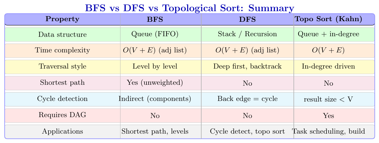
BFS/DFS tracing: Always maintain a queue/stack carefully. Follow the adjacency list order strictly. Commonly asked: what is the BFS/DFS order, what are the timestamps, what type is each edge.
Edge classification: On a directed graph DFS, a back edge means a cycle. On an undirected graph DFS, there are no forward or cross edges, only tree and back edges.
Topological sort: Only on DAGs. Multiple valid orderings may exist. Kahn's algorithm also detects cycles. DFS-based gives reverse of finish time.
Complexity: $O(V+E)$ on adjacency list, $O(V^2)$ on adjacency matrix. Always specify which representation.
BFS shortest path: Only gives shortest in terms of edge count (unweighted graphs). Not for weighted graphs.